Introduction to the vital package

The goal of vital is to allow analysis of demographic data using tidy tools. It works with other tidyverse packages such as dplyr and ggplot2. It also works with the tidyverts packages, tsibble and fable.

library(vital)
library(tsibble)
library(dplyr)
library(ggplot2)

vital objects

The basic data object is a vital, which is time-indexed tibble that contains vital statistics such as births, deaths, population counts, and mortality and fertility rates.

We will use Norwegian data in the following examples. First, let’s remove the “Total” Sex category and collapse the upper ages into a final age group of 100+.

nor <- norway_mortality |>
  filter(Sex != "Total") |>
  collapse_ages(max_age = 100) 
nor
#> # A vital: 24,846 x 6 [1Y]
#> # Key:     Age x Sex [101 x 2]
#>     Year   Age OpenInterval Sex    Population Mortality
#>    <int> <int> <lgl>        <chr>       <dbl>     <dbl>
#>  1  1900     0 FALSE        Female      30070   0.0778 
#>  2  1900     1 FALSE        Female      28960   0.0290 
#>  3  1900     2 FALSE        Female      28043   0.0123 
#>  4  1900     3 FALSE        Female      27019   0.00786
#>  5  1900     4 FALSE        Female      26854   0.00624
#>  6  1900     5 FALSE        Female      25569   0.00538
#>  7  1900     6 FALSE        Female      25534   0.00422
#>  8  1900     7 FALSE        Female      24314   0.00376
#>  9  1900     8 FALSE        Female      24979   0.00380
#> 10  1900     9 FALSE        Female      24428   0.00365
#> # ℹ 24,836 more rows

This example contains data from 1900 to 2022. There are 101 age groups and 2 Sex categories. A vital must have a time “index” variable, and optionally other categorical variables known as “key” variables. Each row must have a unique combination of the index and key variables. Some columns are “vital” variables, such as “Age” and “Sex”.

We can use functions to see which variables are index, key or vital:

index_var(nor)
#> [1] "Year"
key_vars(nor)
#> [1] "Age" "Sex"
vital_vars(nor)
#>          age          sex   population 
#>        "Age"        "Sex" "Population"

Plots

There are autoplot() functions for plotting vital objects. These produce rainbow plots (Hyndman and Shang 2010) where each line represents data for one year, and the variable is plotted against age.

nor |> 
  autoplot(Mortality) + 
  scale_y_log10()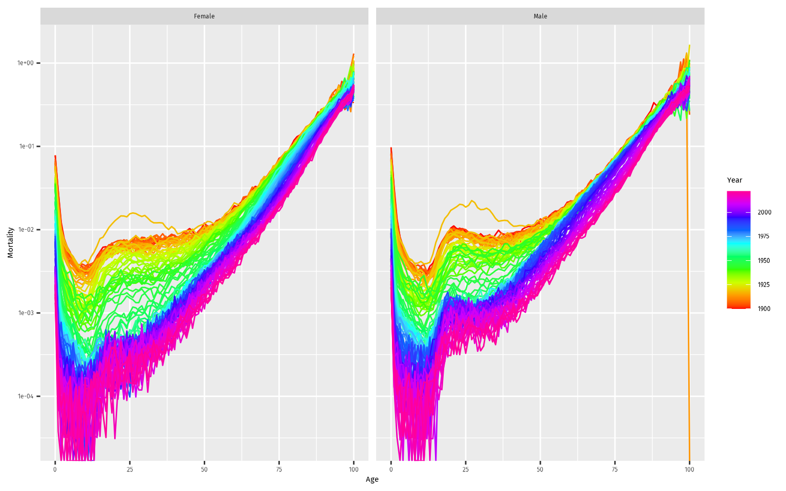

We can use standard ggplot functions to modify the plot as desired. For example, here are population pyramids for all years.

nor |> 
  mutate(Population = if_else(Sex == "Female", -Population, Population)) |>
  autoplot(Population) +
  coord_flip() +
  facet_grid( . ~ Sex, scales = "free_x")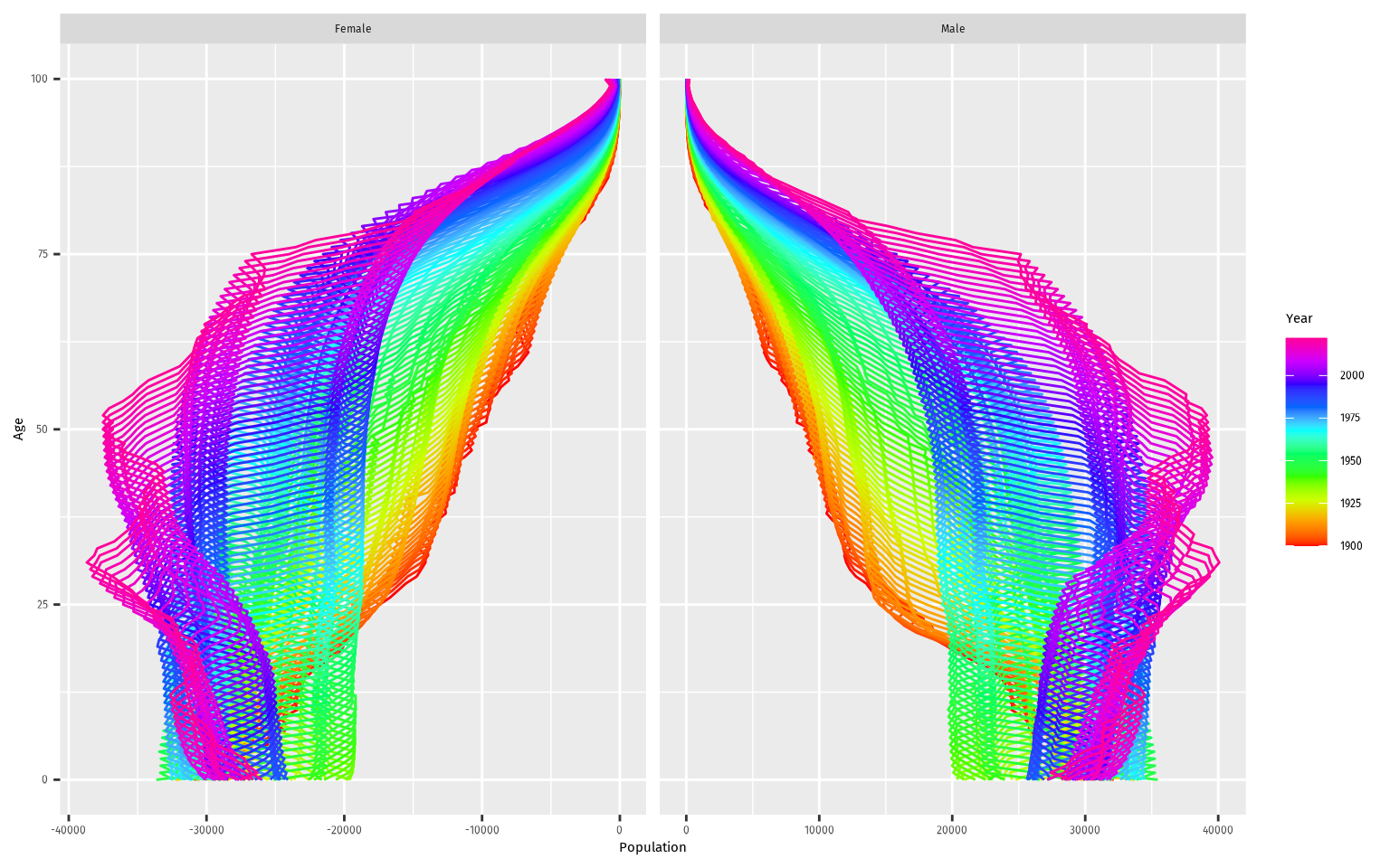

Life tables and life expectancy

Life tables (Chiang 1984) can be produced using the life_table() function. It will produce life tables for each unique combination of the index and key variables other than age.

# Life tables for males and females in Norway in 2000
nor |>
  filter(Year == 2000) |>
  life_table()
#> # A vital: 202 x 13 [?]
#> # Key:     Age x Sex [101 x 2]
#>     Year   Age Sex        mx      qx    lx      dx    Lx    Tx    ex    rx    nx
#>    <int> <int> <chr>   <dbl>   <dbl> <dbl>   <dbl> <dbl> <dbl> <dbl> <dbl> <dbl>
#>  1  2000     0 Fema… 3.28e-3 3.27e-3 1     3.27e-3 0.997  81.4  81.4 0.997     1
#>  2  2000     1 Fema… 2.77e-4 2.77e-4 0.997 2.76e-4 0.997  80.4  80.6 1.00      1
#>  3  2000     2 Fema… 3.09e-4 3.09e-4 0.996 3.08e-4 0.996  79.4  79.7 1.00      1
#>  4  2000     3 Fema… 1.33e-4 1.33e-4 0.996 1.32e-4 0.996  78.4  78.7 1.00      1
#>  5  2000     4 Fema… 1.68e-4 1.68e-4 0.996 1.67e-4 0.996  77.4  77.7 1.00      1
#>  6  2000     5 Fema… 3.30e-5 3.30e-5 0.996 3.29e-5 0.996  76.4  76.7 1.00      1
#>  7  2000     6 Fema… 1.35e-4 1.35e-4 0.996 1.34e-4 0.996  75.4  75.7 1.00      1
#>  8  2000     7 Fema… 1.68e-4 1.68e-4 0.996 1.67e-4 0.996  74.4  74.7 1.00      1
#>  9  2000     8 Fema… 6.70e-5 6.70e-5 0.996 6.67e-5 0.995  73.4  73.7 1.00      1
#> 10  2000     9 Fema… 1.97e-4 1.97e-4 0.995 1.96e-4 0.995  72.4  72.7 1.00      1
#> # ℹ 192 more rows
#> # ℹ 1 more variable: ax <dbl>

Life expectancy ( $e_x$ with $x=0$ by default) is computed using life_expectancy():

# Life expectancy for males and females in Norway
nor |>
  life_expectancy() |>
  ggplot(aes(x = Year, y = ex, color = Sex)) +
  geom_line()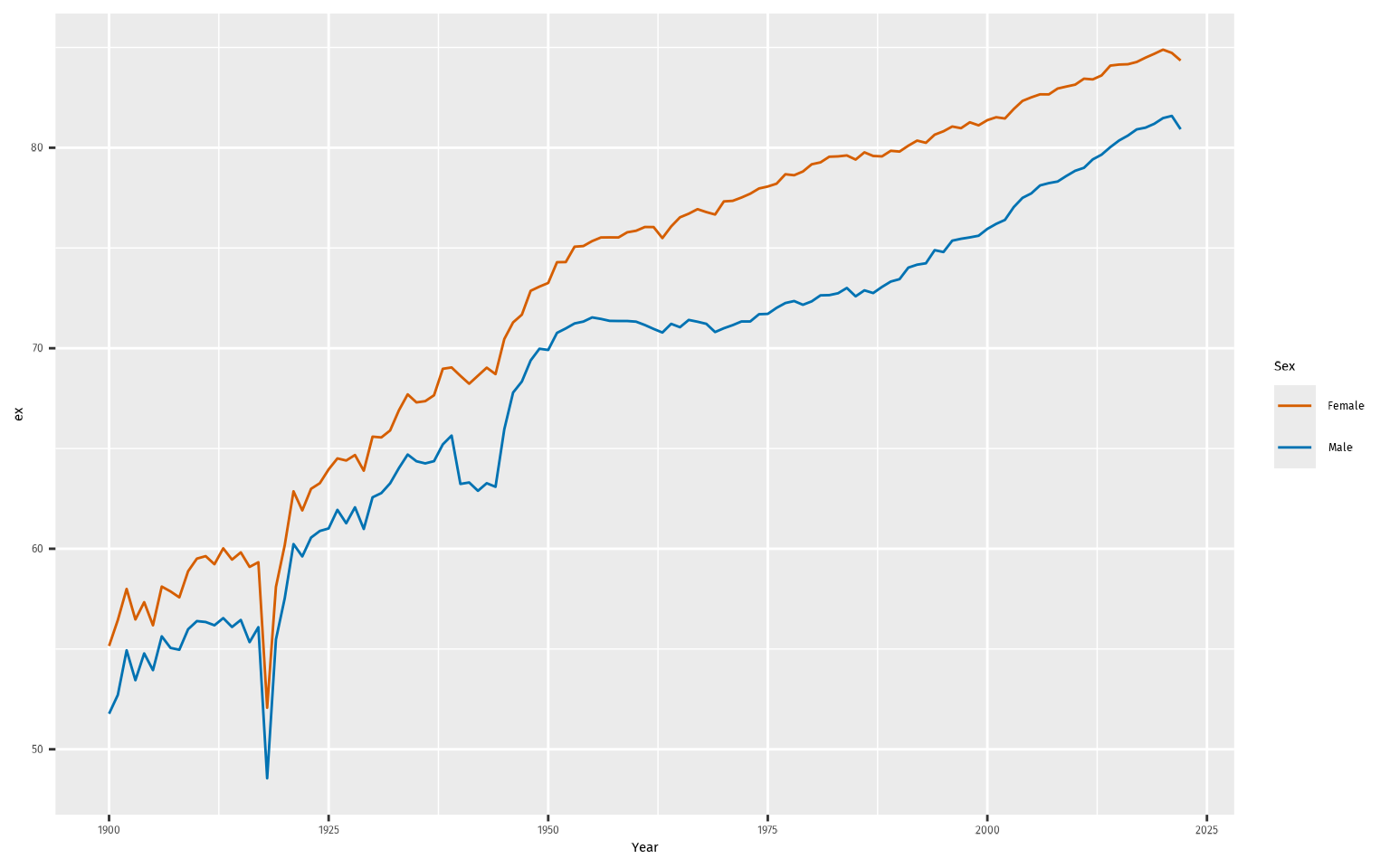

Smoothing

Several smoothing functions are provided: smooth_spline(), smooth_mortality(), smooth_fertility(), and smooth_loess(), each smoothing across the age variable for each year. The methods used in smooth_mortality() and smooth_fertility() are described in Hyndman and Ullah (2007).

# Smoothed data
nor |>
  filter(Year == 1967) |>
  smooth_mortality(Mortality) |>
  autoplot(Mortality) +
  geom_line(aes(y = .smooth), col = "#0072B2") +
  ylab("Mortality rate") +
  scale_y_log10()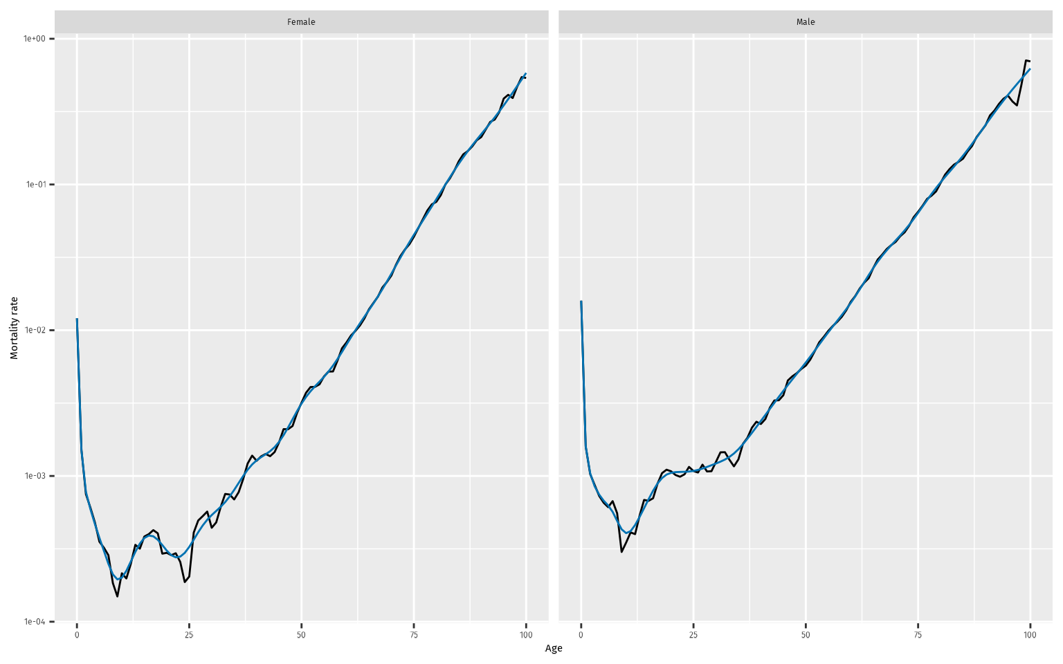

Lee-Carter models

Lee-Carter models (Lee and Carter 1992) are estimated using the LC() function which must be called within a model() function:

# Lee-Carter model
lc <- nor |>
  model(lee_carter = LC(log(Mortality)))
lc
#> # A mable: 2 x 2
#> # Key:     Sex [2]
#>   Sex    lee_carter
#>   <chr>     <model>
#> 1 Female       <LC>
#> 2 Male         <LC>

Models are fitted for all combinations of key variables excluding age. To see the details for a specific model, use the report() function.

lc |> 
  filter(Sex == "Female") |> 
  report()
#> Series: Mortality 
#> Model: LC 
#> Transformation: log(Mortality) 
#> 
#> Options:
#>   Adjust method: dt
#>   Jump choice: fit
#> 
#> Age functions
#> # A tibble: 101 × 3
#>     Age    ax     bx
#>   <int> <dbl>  <dbl>
#> 1     0 -4.32 0.0154
#> 2     1 -6.15 0.0224
#> 3     2 -6.76 0.0192
#> 4     3 -7.13 0.0187
#> 5     4 -7.16 0.0164
#> # ℹ 96 more rows
#> 
#> Time coefficients
#> # A tsibble: 123 x 2 [1Y]
#>    Year    kt
#>   <int> <dbl>
#> 1  1900  115.
#> 2  1901  110.
#> 3  1902  107.
#> 4  1903  113.
#> 5  1904  111.
#> # ℹ 118 more rows
#> 
#> Time series model: RW w/ drift 
#> 
#> Variance explained: 66.95%

The results can be plotted.

autoplot(lc)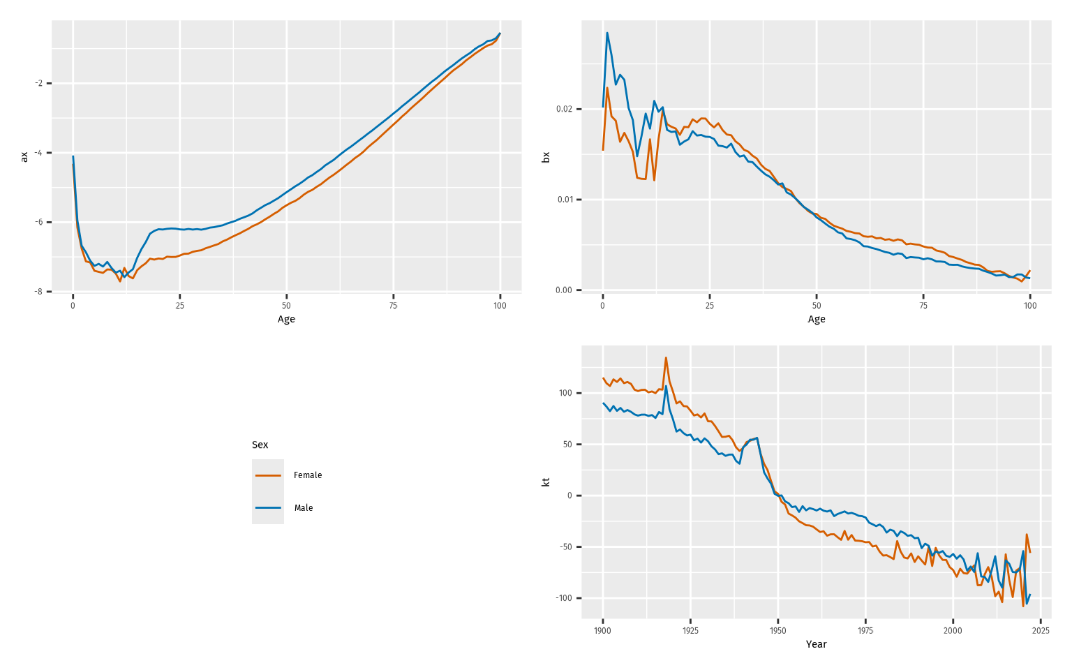

The components can be extracted.

age_components(lc)
#> # A tibble: 202 × 4
#>    Sex      Age    ax     bx
#>    <chr>  <int> <dbl>  <dbl>
#>  1 Female     0 -4.32 0.0154
#>  2 Female     1 -6.15 0.0224
#>  3 Female     2 -6.76 0.0192
#>  4 Female     3 -7.13 0.0187
#>  5 Female     4 -7.16 0.0164
#>  6 Female     5 -7.40 0.0174
#>  7 Female     6 -7.43 0.0165
#>  8 Female     7 -7.46 0.0153
#>  9 Female     8 -7.36 0.0124
#> 10 Female     9 -7.37 0.0123
#> # ℹ 192 more rows
time_components(lc)
#> # A tsibble: 246 x 3 [1Y]
#> # Key:       Sex [2]
#>    Sex     Year    kt
#>    <chr>  <int> <dbl>
#>  1 Female  1900  115.
#>  2 Female  1901  110.
#>  3 Female  1902  107.
#>  4 Female  1903  113.
#>  5 Female  1904  111.
#>  6 Female  1905  114.
#>  7 Female  1906  110.
#>  8 Female  1907  111.
#>  9 Female  1908  109.
#> 10 Female  1909  103.
#> # ℹ 236 more rows

Forecasts are obtained using the forecast() function

# Forecasts from Lee-Carter model
lc |>
  forecast(h = 20) 
#> # A vital fable: 4,040 x 6 [1Y]
#> # Key:           Age x (Sex, .model) [101 x 2]
#>    Sex    .model      Year   Age         Mortality   .mean
#>    <chr>  <chr>      <dbl> <int>            <dist>   <dbl>
#>  1 Female lee_carter  2023     0 t(N(-5.2, 0.033)) 0.00560
#>  2 Female lee_carter  2024     0 t(N(-5.2, 0.066)) 0.00557
#>  3 Female lee_carter  2025     0 t(N(-5.2, 0.099)) 0.00554
#>  4 Female lee_carter  2026     0  t(N(-5.3, 0.13)) 0.00551
#>  5 Female lee_carter  2027     0  t(N(-5.3, 0.17)) 0.00548
#>  6 Female lee_carter  2028     0   t(N(-5.3, 0.2)) 0.00545
#>  7 Female lee_carter  2029     0  t(N(-5.3, 0.24)) 0.00542
#>  8 Female lee_carter  2030     0  t(N(-5.4, 0.27)) 0.00539
#>  9 Female lee_carter  2031     0  t(N(-5.4, 0.31)) 0.00536
#> 10 Female lee_carter  2032     0  t(N(-5.4, 0.35)) 0.00533
#> # ℹ 4,030 more rows

The forecasts are returned as a distribution column (here transformed normal because of the log transformation used in the model). The .mean column gives the point forecasts equal to the mean of the distribution column.

Functional data models

Functional data models (Hyndman and Ullah 2007) can be estimated in a similar way to Lee-Carter models, but with an additional smoothing step, then modelling with LC replaced by FDM.

# FDM model
fdm <- nor |> 
  smooth_mortality(Mortality) |> 
  model(hu = FDM(log(.smooth)))
fc_fdm <- fdm |>
  forecast(h = 20) 
autoplot(fc_fdm) +
  scale_y_log10()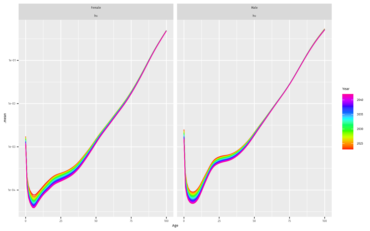

Functional data models have multiple principal components, rather than the single factor used in Lee-Carter models.

fdm |>
  autoplot(show_order = 3)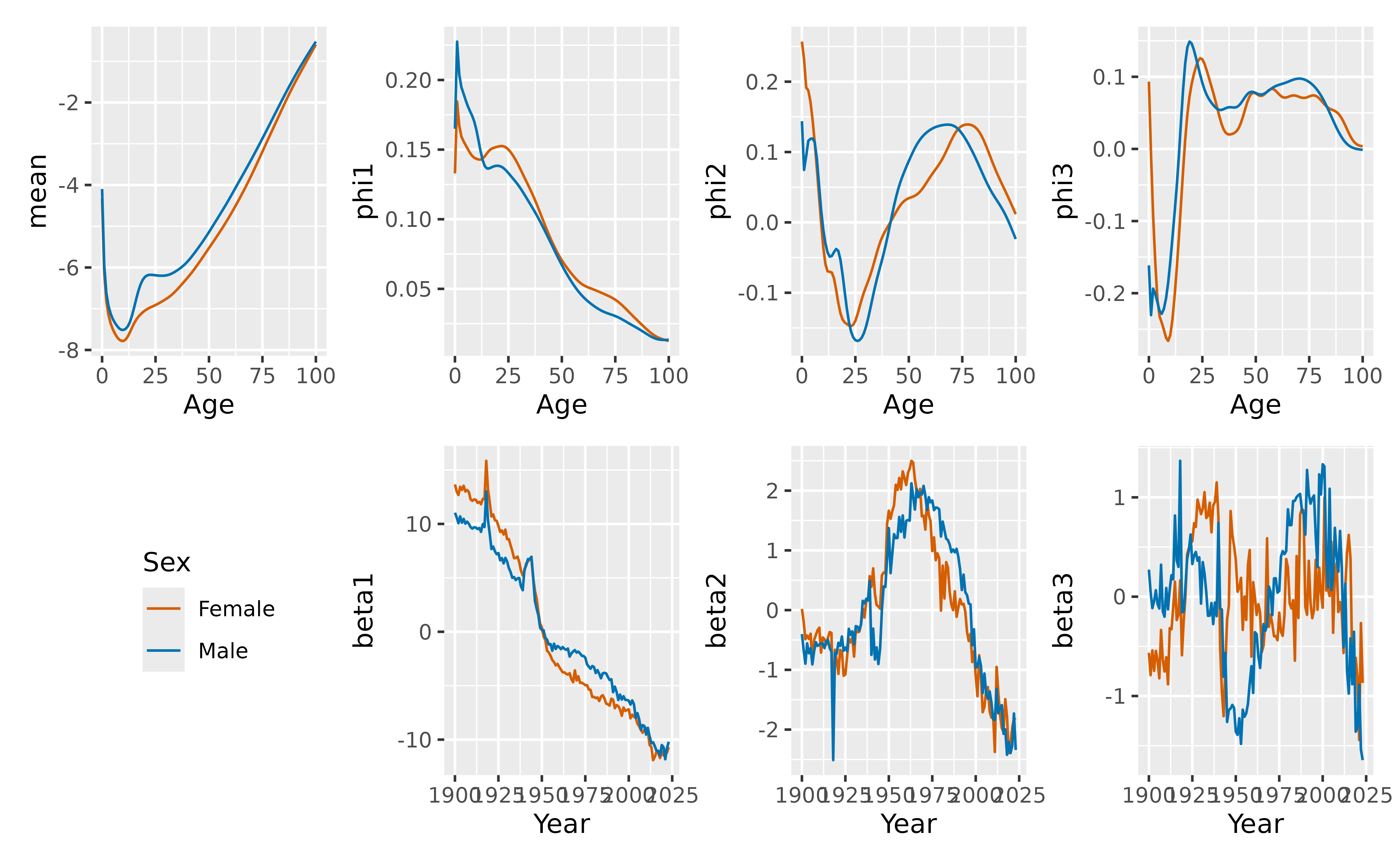

By default, six factors are estimated using FDM(). Here we have chosen to plot only the first three.

The components can be extracted.

age_components(fdm)
#> # A tibble: 202 × 9
#>    Sex      Age  mean  phi1    phi2    phi3    phi4     phi5    phi6
#>    <chr>  <dbl> <dbl> <dbl>   <dbl>   <dbl>   <dbl>    <dbl>   <dbl>
#>  1 Female     0 -4.32 0.132 0.256    0.0944 -0.0742 -0.0636   0.0492
#>  2 Female     1 -6.11 0.185 0.239    0.0104 -0.214  -0.123    0.397 
#>  3 Female     2 -6.80 0.168 0.197   -0.0780 -0.232   0.00728  0.0667
#>  4 Female     3 -7.14 0.160 0.192   -0.146  -0.255   0.0774  -0.0286
#>  5 Female     4 -7.34 0.156 0.180   -0.198  -0.280   0.0803  -0.112 
#>  6 Female     5 -7.48 0.153 0.150   -0.225  -0.262   0.0865  -0.225 
#>  7 Female     6 -7.59 0.151 0.112   -0.240  -0.177   0.0723  -0.249 
#>  8 Female     7 -7.68 0.148 0.0733  -0.253  -0.0577  0.0203  -0.158 
#>  9 Female     8 -7.74 0.146 0.0372  -0.265   0.0471 -0.0547  -0.0237
#> 10 Female     9 -7.77 0.144 0.00134 -0.269   0.123  -0.131    0.0837
#> # ℹ 192 more rows
time_components(fdm)
#> # A tsibble: 246 x 9 [1Y]
#> # Key:       Sex [2]
#>    Sex     Year  mean beta1   beta2  beta3   beta4   beta5  beta6
#>    <chr>  <int> <dbl> <dbl>   <dbl>  <dbl>   <dbl>   <dbl>  <dbl>
#>  1 Female  1900     1  13.6  0.0330 -0.563  0.0921 -0.0698 -0.317
#>  2 Female  1901     1  12.9 -0.171  -0.785  0.0404 -0.116  -0.248
#>  3 Female  1902     1  12.6 -0.474  -0.536 -0.0642 -0.151  -0.503
#>  4 Female  1903     1  13.4 -0.403  -0.739 -0.0355 -0.0865 -0.108
#>  5 Female  1904     1  13.1 -0.468  -0.547  0.171  -0.220  -0.389
#>  6 Female  1905     1  13.5 -0.374  -0.635 -0.0485 -0.0103 -0.120
#>  7 Female  1906     1  12.9 -0.866  -0.820  0.0496 -0.124  -0.223
#>  8 Female  1907     1  13.1 -0.490  -0.344  0.260  -0.103  -0.213
#>  9 Female  1908     1  12.9 -0.407  -0.636  0.0854 -0.171  -0.201
#> 10 Female  1909     1  12.2 -0.329  -0.753  0.0104 -0.130  -0.381
#> # ℹ 236 more rows

Coherent functional data models

A coherent functional data model (Hyndman, Booth, and Yasmeen 2013), is obtained by first computing the sex-products and sex-ratios of the smoothed mortality data. Then a functional data model is fitted to the smoothed data, forecasts are obtained, and the product/ratio transformation is reversed. The following code shows the steps.

fdm_coherent <- nor |> 
  smooth_mortality(Mortality) |> 
  make_pr(.smooth) |>
  model(hby = FDM(log(.smooth), coherent = TRUE))
fc_coherent <- fdm_coherent |>
  forecast(h = 20) |>
  undo_pr(.smooth)
fc_coherent
#> # A vital fable: 4,040 x 6 [1Y]
#> # Key:           Age x (Sex, .model) [101 x 2]
#>     Year   Age Sex    .model      .smooth     .mean
#>    <dbl> <dbl> <chr>  <chr>        <dist>     <dbl>
#>  1  2023     0 Female hby    sample[2000] 0.00180  
#>  2  2023     1 Female hby    sample[2000] 0.000219 
#>  3  2023     2 Female hby    sample[2000] 0.000138 
#>  4  2023     3 Female hby    sample[2000] 0.000110 
#>  5  2023     4 Female hby    sample[2000] 0.0000958
#>  6  2023     5 Female hby    sample[2000] 0.0000892
#>  7  2023     6 Female hby    sample[2000] 0.0000866
#>  8  2023     7 Female hby    sample[2000] 0.0000859
#>  9  2023     8 Female hby    sample[2000] 0.0000886
#> 10  2023     9 Female hby    sample[2000] 0.0000930
#> # ℹ 4,030 more rows

Here, make_pr() makes the product-ratios, while undo_pr() undoes them.

The argument coherent = TRUE in FDM() ensures that the ARIMA models fitted to the coefficients are stationary when applied to the sex-ratios.

References

Chiang, Chin Long. 1984. The Life Table and Its Applications. Malabar: Robert E Krieger Publishing Company.

Hyndman, Rob J, Heather Booth, and Farah Yasmeen. 2013. “Coherent Mortality Forecasting: The Product-Ratio Method with Functional Time Series Models.” Demography 50 (1): 261–83.

Hyndman, Rob J, and Han Lin Shang. 2010. “Rainbow Plots, Bagplots, and Boxplots for Functional Data.” Journal of Computational and Graphical Statistics 19 (1): 29–45. https://robjhyndman.com/publications/rainbow-fda/.

Hyndman, Rob J, and Md Shahid Ullah. 2007. “Robust Forecasting of Mortality and Fertility Rates: A Functional Data Approach.” Computational Statistics & Data Analysis 51 (10): 4942–56. https://robjhyndman.com/publications/funcfor/.

Lee, Ronald D, and Lawrence R Carter. 1992. “Modeling and Forecasting US Mortality.” Journal of the American Statistical Association 87 (419): 659–71.

Rob J Hyndman