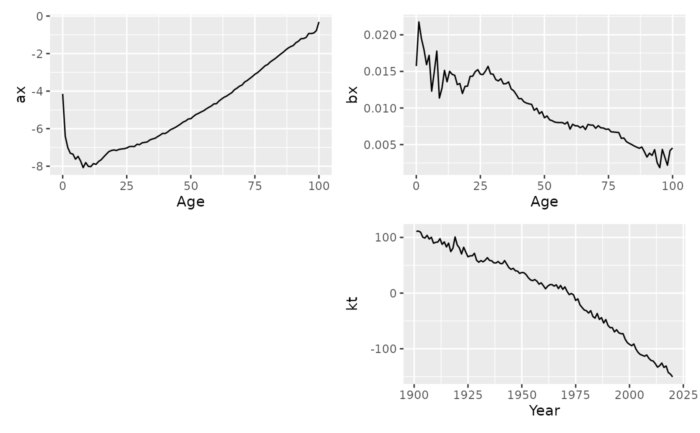
Lee-Carter model

Lee-Carter model of mortality or fertility rates. LC() returns a Lee-Carter model applied to the formula's response variable as a function of age. This produces a standard Lee-Carter model by default, although many other options are available. Missing rates are set to the geometric mean rate for the relevant age.

Usage

LC(
  formula,
  adjust = c("dt", "dxt", "e0", "none"),
  jump_choice = c("fit", "actual"),
  scale = FALSE,
  ...
)

Arguments

formula

Model specification. It should include the log of the variable to be modelled. See the examples.

adjust

method to use for adjustment of coefficients \(k_t\). Possibilities are "dt" (Lee-Carter method, the default), "dxt" (BMS method), "e0" (Lee-Miller method based on life expectancy) and "none".

jump_choice

Method used for computation of jump-off point for forecasts. Possibilities: "actual" (use actual rates from final year) and "fit" (use fitted rates). The original Lee-Carter method used "fit" (the default), but Lee and Miller (2001) and most other authors prefer "actual".

scale

If TRUE, bx and kt are rescaled so that kt has drift parameter = 1.

...

Not used.

Value

A model specification.

References

Basellini, U, Camarda, C G, and Booth, H (2022) Thirty years on: A review of the Lee-Carter method for forecasting mortality. International Journal of Forecasting, 39(3), 1033-1049.

Booth, H., Maindonald, J., and Smith, L. (2002) Applying Lee-Carter under conditions of variable mortality decline. Population Studies, 56, 325-336.

Lee, R D, and Carter, L R (1992) Modeling and forecasting US mortality. Journal of the American Statistical Association, 87, 659-671.

Lee R D, and Miller T (2001). Evaluating the performance of the Lee-Carter method for forecasting mortality. Demography, 38(4), 537–549.

Author

Rob J Hyndman

Examples

lc <- aus_mortality |>
  dplyr::filter(State == "Victoria", Sex == "female") |>
  model(lee_carter = LC(log(Mortality)))
report(lc)
#> Series: Mortality 
#> Model: LC 
#> Transformation: log(Mortality) 
#> 
#> Options:
#>   Adjust method: dt
#>   Jump choice: fit
#> 
#> Age functions
#> # A tibble: 101 × 3
#>     Age    ax     bx
#>   <int> <dbl>  <dbl>
#> 1     0 -4.15 0.0157
#> 2     1 -6.40 0.0218
#> 3     2 -7.01 0.0195
#> 4     3 -7.32 0.0180
#> 5     4 -7.36 0.0159
#> # ℹ 96 more rows
#> 
#> Time coefficients
#> # A tsibble: 120 x 2 [1Y]
#>    Year    kt
#>   <int> <dbl>
#> 1  1901 111. 
#> 2  1902 111. 
#> 3  1903 109. 
#> 4  1904 100. 
#> 5  1905  98.8
#> # ℹ 115 more rows
#> 
#> Time series model: RW w/ drift 
#> 
#> Variance explained: 72.99%
autoplot(lc)