Functional data model

Functional data model of mortality or fertility rates as a function of age. FDM() returns a functional data model applied to the formula's response variable as a function of age.

Usage

FDM(formula, order = 6, ts_model_fn = fable::ARIMA, coherent = FALSE, ...)

Arguments

formula

Model specification.

order

Number of principal components to fit.

ts_model_fn

Univariate time series modelling function for the coefficients. Any model that works with the fable package is ok. Default is fable::ARIMA().

coherent

If TRUE, fitted models are stationary, other than for the case of a key variable taking the value geometric_mean or mean. This is designed to work with vitals produced using make_pr() and make_sd. Default is FALSE. It only works when ts_model_fn is ARIMA().

...

Not used.

Value

A model specification.

References

Hyndman, R. J., and Ullah, S. (2007) Robust forecasting of mortality and fertility rates: a functional data approach. Computational Statistics & Data Analysis, 5, 4942-4956. https://robjhyndman.com/publications/funcfor/

Hyndman, R. J., Booth, H., & Yasmeen, F. (2013). Coherent mortality forecasting: the product-ratio method with functional time series models. Demography, 50(1), 261-283. https://robjhyndman.com/publications/coherentfdm/

Author

Rob J Hyndman

Examples

hu <- norway_mortality |>
  dplyr::filter(Sex == "Female", Year > 2010) |>
  smooth_mortality(Mortality) |>
  model(hyndman_ullah = FDM(log(.smooth)))
report(hu)
#> Series: .smooth 
#> Model: FDM 
#> Transformation: log(.smooth) 
#> 
#> Basis functions
#> # A tibble: 111 × 8
#>     Age  mean    phi1    phi2  phi3     phi4     phi5    phi6
#>   <dbl> <dbl>   <dbl>   <dbl> <dbl>    <dbl>    <dbl>   <dbl>
#> 1     0 -6.27 -0.0470  0.153  0.107  0.220    0.00196 -0.299 
#> 2     1 -8.51  0.167   0.107  0.295  0.00735 -0.410   -0.269 
#> 3     2 -9.00  0.170   0.0341 0.295 -0.00474 -0.314   -0.195 
#> 4     3 -9.22  0.155  -0.0284 0.298 -0.0733  -0.121   -0.0204
#> 5     4 -9.33  0.119  -0.0878 0.298 -0.125    0.0290   0.103 
#> # ℹ 106 more rows
#> 
#> Coefficients
#> # A tsibble: 13 x 8 [1Y]
#>    Year  mean  beta1 beta2  beta3  beta4   beta5   beta6
#>   <int> <dbl>  <dbl> <dbl>  <dbl>  <dbl>   <dbl>   <dbl>
#> 1  2011     1  2.06  0.297 -0.562 0.0844  0.164   0.119 
#> 2  2012     1  0.356 0.135  0.943 0.543   0.314  -0.134 
#> 3  2013     1  0.126 0.662  0.334 0.437  -0.0629  0.0955
#> 4  2014     1 -0.892 0.729 -0.246 0.175   0.258   0.0968
#> 5  2015     1 -0.652 0.678 -0.418 0.128  -0.410   0.0857
#> # ℹ 8 more rows
#> 
#> Time series models
#>    beta1 : ARIMA(0,0,0) 
#>    beta2 : ARIMA(1,0,0) 
#>    beta3 : ARIMA(0,0,0) 
#>    beta4 : ARIMA(0,0,0) 
#>    beta5 : ARIMA(0,0,0) 
#>    beta6 : ARIMA(0,0,0) 
#> 
#> Variance explained
#>   34.57 + 23.46 + 18.78 + 13.54 + 5.59 + 1.5 = 97.45%
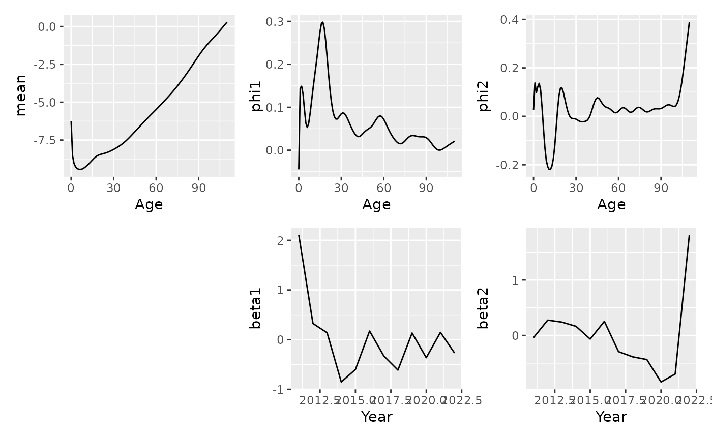
autoplot(hu)