Naive and Random Walk Forecasts

Returns forecasts and prediction intervals for a generalized random walk model. rwf() is a convenience function that combines rw_model() and forecast(). naive() is a wrapper to rwf() with drift=FALSE and lag=1, while snaive() is a wrapper to rwf() with drift=FALSE and lag=frequency(y).

Usage

# S3 method for class 'rw_model'
forecast(
  object,
  h = 10,
  level = c(80, 95),
  fan = FALSE,
  lambda = NULL,
  simulate = FALSE,
  bootstrap = FALSE,
  npaths = 5000,
  biasadj = FALSE,
  ...
)

rwf(
  y,
  h = 10,
  drift = FALSE,
  level = c(80, 95),
  fan = FALSE,
  lambda = NULL,
  biasadj = FALSE,
  lag = 1,
  ...,
  x = y
)

naive(
  y,
  h = 10,
  level = c(80, 95),
  fan = FALSE,
  lambda = NULL,
  biasadj = FALSE,
  ...,
  x = y
)

snaive(
  y,
  h = 2 * frequency(x),
  level = c(80, 95),
  fan = FALSE,
  lambda = NULL,
  biasadj = FALSE,
  ...,
  x = y
)

Arguments

object: An object of class rw_model returned by rw_model().
h: Number of periods for forecasting. Default value is twice the largest seasonal period (for seasonal data) or ten (for non-seasonal data).
level: Confidence levels for prediction intervals.
fan: If TRUE, level is set to seq(51, 99, by = 3). This is suitable for fan plots.
lambda: Box-Cox transformation parameter. If lambda = "auto", then a transformation is automatically selected using BoxCox.lambda. The transformation is ignored if NULL. Otherwise, data transformed before model is estimated.
simulate: If TRUE, prediction intervals are produced by simulation rather than using analytic formulae. Errors are assumed to be normally distributed.
bootstrap: If TRUE, then prediction intervals are produced by simulation using resampled errors (rather than normally distributed errors).
npaths: Number of sample paths used in computing simulated prediction intervals.
biasadj: Use adjusted back-transformed mean for Box-Cox transformations. If transformed data is used to produce forecasts and fitted values, a regular back transformation will result in median forecasts. If biasadj is TRUE, an adjustment will be made to produce mean forecasts and fitted values.
...: Additional arguments not used.
y: a numeric vector or univariate time series of class ts
drift: Logical flag. If TRUE, fits a random walk with drift model.
lag: Lag parameter. lag = 1 corresponds to a standard random walk (giving naive forecasts if drift = FALSE or drift forecasts if drift = TRUE), while lag = m corresponds to a seasonal random walk where m is the seasonal period (giving seasonal naive forecasts if drift = FALSE).
x: Deprecated. Included for backwards compatibility.

Value

An object of class forecast.

Details

The model assumes that

$$Y_t = Y_{t-p} + c + \varepsilon_{t}$$

where $p$ is the lag parameter, $c$ is the drift parameter, and $\varepsilon_t\sim N(0,\sigma^2)$ are iid.

The model without drift has $c=0$. In the model with drift, $c$ is estimated by the sample mean of the differences $Y_t - Y_{t-p}$.

If $p=1$, this is equivalent to an ARIMA(0,1,0) model with an optional drift coefficient. For $p>1$, it is equivalent to an ARIMA(0,0,0)(0,1,0)p model.

The forecasts are given by

$$Y_{T+h|T}= Y_{T+h-p(k+1)} + ch$$

where $k$ is the integer part of $(h-1)/p$. For a regular random walk, $p=1$ and $c=0$, so all forecasts are equal to the last observation. Forecast standard errors allow for uncertainty in estimating the drift parameter (unlike the corresponding forecasts obtained by fitting an ARIMA model directly).

The generic accessor functions stats::fitted() and stats::residuals() extract useful features of the object returned.

forecast class

An object of class forecast is a list usually containing at least the following elements:

model: A list containing information about the fitted model
method: The name of the forecasting method as a character string
mean: Point forecasts as a time series
lower: Lower limits for prediction intervals
upper: Upper limits for prediction intervals
level: The confidence values associated with the prediction intervals
x: The original time series.
residuals: Residuals from the fitted model. For models with additive errors, the residuals will be x minus the fitted values.
fitted: Fitted values (one-step forecasts)

The function summary can be used to obtain and print a summary of the results, while the functions plot and autoplot produce plots of the forecasts and prediction intervals. The generic accessors functions fitted.values and residuals extract various useful features from the underlying model.

Author

Rob J Hyndman

Examples

# Three ways to do the same thing
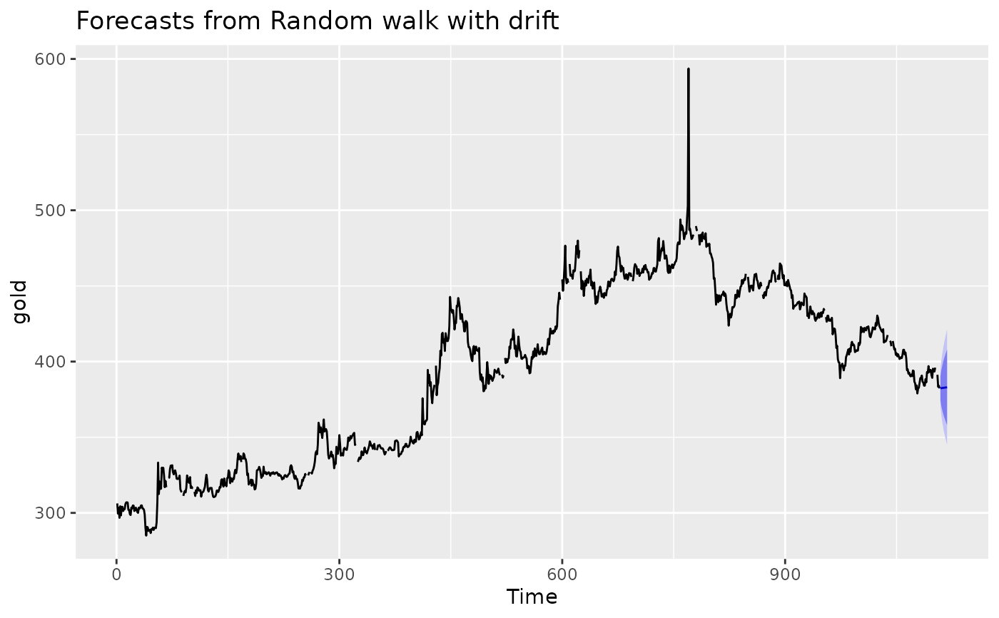
gold_model <- rw_model(gold)
gold_fc1 <- forecast(gold_model, h = 50)
gold_fc2 <- rwf(gold, h = 50)
gold_fc3 <- naive(gold, h = 50)

# Plot the forecasts
autoplot(gold_fc1)


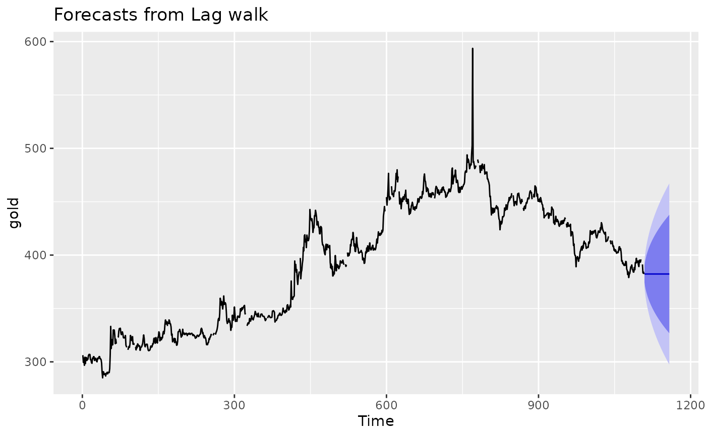# Drift forecasts
rwf(gold, drift = TRUE) |> autoplot()


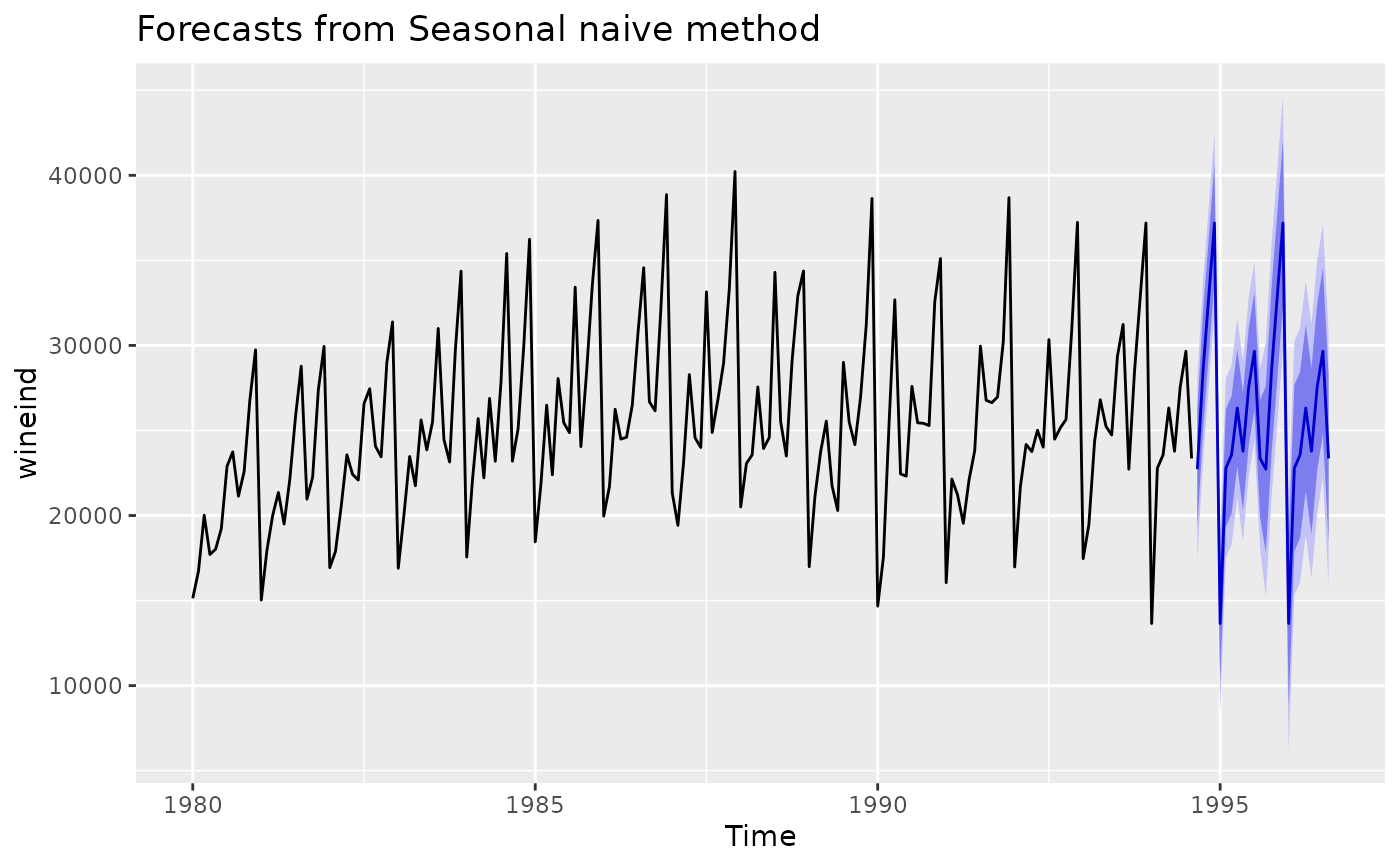
# Seasonal naive forecasts
snaive(wineind) |> autoplot()