Fit ARIMA model to univariate time series

Largely a wrapper for the arima function in the stats package. The main difference is that this function allows a drift term. It is also possible to take an ARIMA model from a previous call to Arima and re-apply it to the data y.

Usage

Arima(
  y,
  order = c(0, 0, 0),
  seasonal = c(0, 0, 0),
  xreg = NULL,
  include.mean = TRUE,
  include.drift = FALSE,
  include.constant,
  lambda = model$lambda,
  biasadj = FALSE,
  method = c("CSS-ML", "ML", "CSS"),
  model = NULL,
  x = y,
  ...
)

Arguments

y: a univariate time series of class ts.
order: A specification of the non-seasonal part of the ARIMA model: the three components (p, d, q) are the AR order, the degree of differencing, and the MA order.
seasonal: A specification of the seasonal part of the ARIMA model, plus the period (which defaults to frequency(y)). This should be a list with components order and period, but a specification of just a numeric vector of length 3 will be turned into a suitable list with the specification as the order.
xreg: Optionally, a numerical vector or matrix of external regressors, which must have the same number of rows as y. It should not be a data frame.
include.mean: Should the ARIMA model include a mean term? The default is TRUE for undifferenced series, FALSE for differenced ones (where a mean would not affect the fit nor predictions).
include.drift: Should the ARIMA model include a linear drift term? (i.e., a linear regression with ARIMA errors is fitted.) The default is FALSE.
include.constant: If TRUE, then include.mean is set to be TRUE for undifferenced series and include.drift is set to be TRUE for differenced series. Note that if there is more than one difference taken, no constant is included regardless of the value of this argument. This is deliberate as otherwise quadratic and higher order polynomial trends would be induced.
lambda: Box-Cox transformation parameter. If lambda="auto", then a transformation is automatically selected using BoxCox.lambda. The transformation is ignored if NULL. Otherwise, data transformed before model is estimated.
biasadj: Use adjusted back-transformed mean for Box-Cox transformations. If transformed data is used to produce forecasts and fitted values, a regular back transformation will result in median forecasts. If biasadj is TRUE, an adjustment will be made to produce mean forecasts and fitted values.
method: Fitting method: maximum likelihood or minimize conditional sum-of-squares. The default (unless there are missing values) is to use conditional-sum-of-squares to find starting values, then maximum likelihood.
model: Output from a previous call to Arima. If model is passed, this same model is fitted to y without re-estimating any parameters.
x: Deprecated. Included for backwards compatibility.
...: Additional arguments to be passed to arima.

Value

See the arima function in the stats package. The additional objects returned are

x: The time series data
xreg: The regressors used in fitting (when relevant).
sigma2: The bias adjusted MLE of the innovations variance.

Details

The fitted model is a regression with ARIMA(p,d,q) errors

$$y_t = c + \beta' x_t + z_t$$

where $x_t$ is a vector of regressors at time $t$ and $z_t$ is an ARMA(p,d,q) error process. If there are no regressors, and $d=0$, then c is an estimate of the mean of $y_t$. For more information, see Hyndman & Athanasopoulos (2018). For details of the estimation algorithm, see the arima function in the stats package.

References

Hyndman, R.J. and Athanasopoulos, G. (2018) "Forecasting: principles and practice", 2nd ed., OTexts, Melbourne, Australia. https://OTexts.com/fpp2/.

Author

Rob J Hyndman

Examples

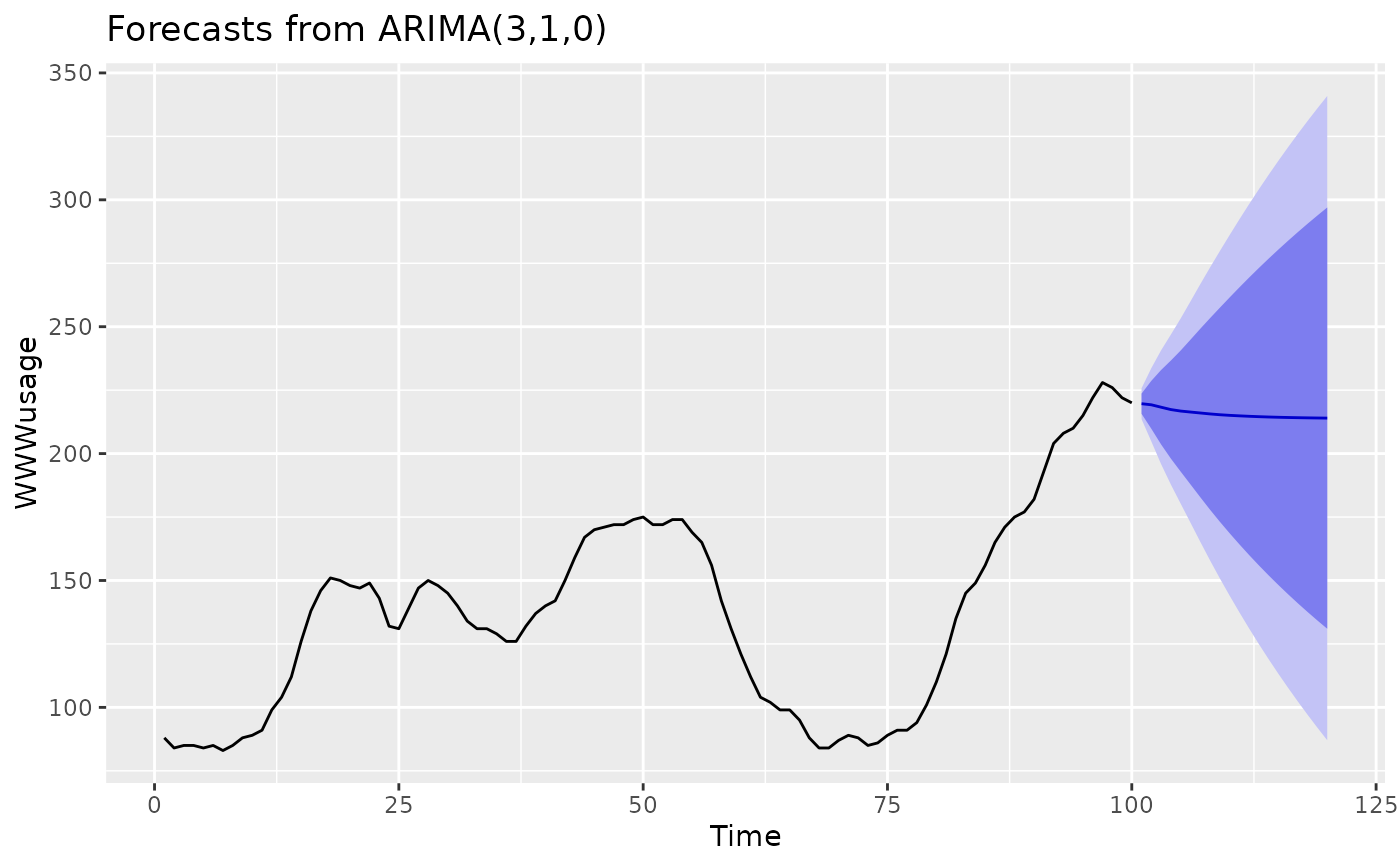
library(ggplot2)
WWWusage %>%
  Arima(order=c(3,1,0)) %>%
  forecast(h=20) %>%
  autoplot


# Fit model to first few years of AirPassengers data
air.model <- Arima(window(AirPassengers,end=1956+11/12),order=c(0,1,1),
                   seasonal=list(order=c(0,1,1),period=12),lambda=0)
plot(forecast(air.model,h=48))
lines(AirPassengers)


# Apply fitted model to later data
air.model2 <- Arima(window(AirPassengers,start=1957),model=air.model)

# Forecast accuracy measures on the log scale.
# in-sample one-step forecasts.
accuracy(air.model)
#>                     ME    RMSE      MAE       MPE     MAPE      MASE       ACF1
#> Training set 0.3576253 7.89734 5.788344 0.1458472 2.670181 0.1982148 0.05807465
# out-of-sample one-step forecasts.
accuracy(air.model2)
#>                     ME     RMSE     MAE        MPE     MAPE      MASE
#> Training set 0.5159268 12.13132 8.14054 0.07949083 1.900931 0.2266508
#>                    ACF1
#> Training set -0.2166661
# out-of-sample multi-step forecasts
accuracy(forecast(air.model,h=48,lambda=NULL),
         log(window(AirPassengers,start=1957)))
#>                       ME      RMSE        MAE        MPE     MAPE      MASE
#> Training set  0.35762533 7.8973404 5.78834425  0.1458472 2.670181 0.1982148
#> Test set     -0.08403416 0.1031891 0.08801596 -1.3982000 1.463555 0.0030140
#>                    ACF1 Theil's U
#> Training set 0.05807465        NA
#> Test set     0.75730561 0.9290965