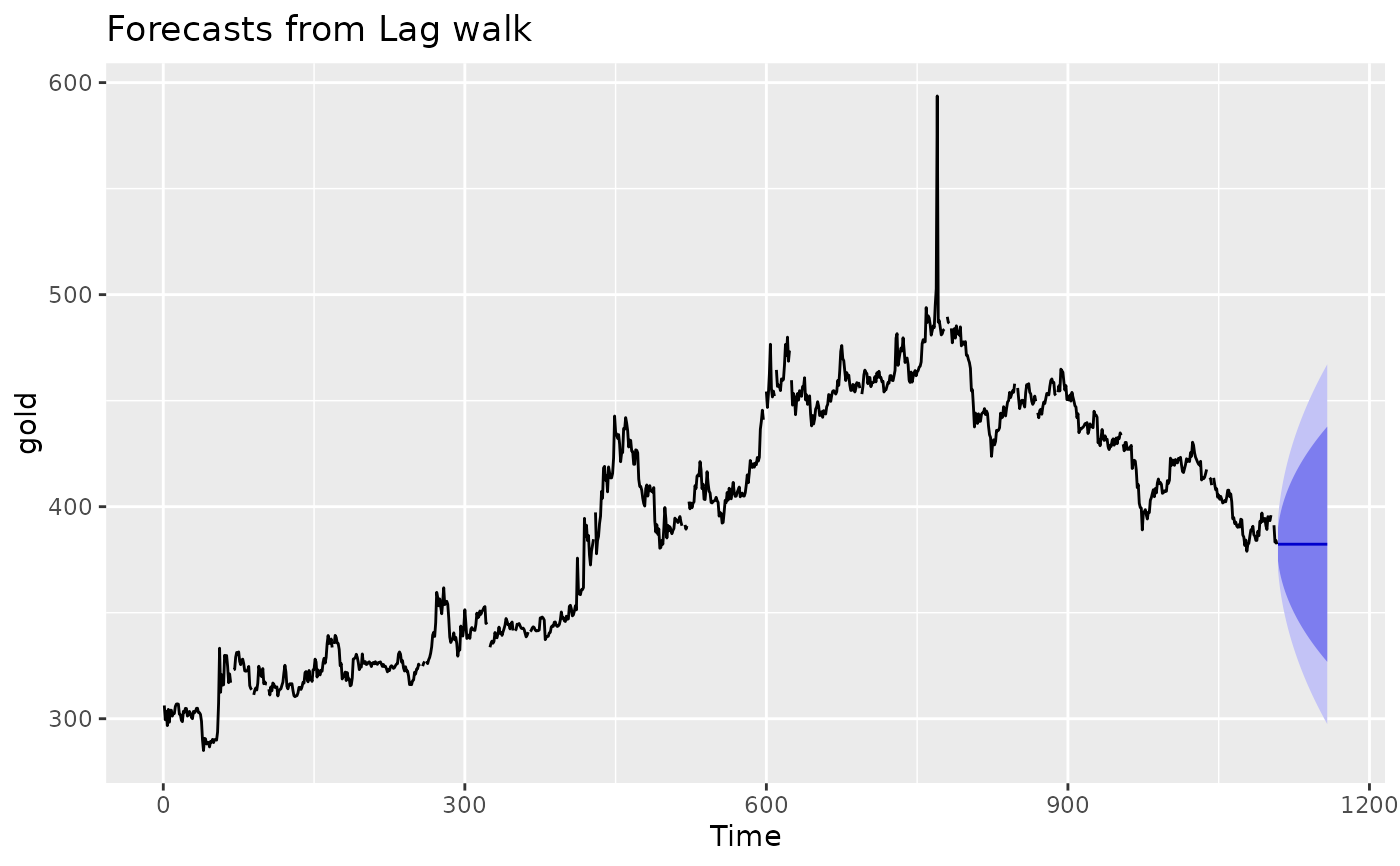
Fit a generalized random walk with Gaussian errors (and optional drift) to a univariate time series.
Arguments
- y
a numeric vector or univariate time series of class
ts- lag
Lag parameter.
lag = 1corresponds to a standard random walk (giving naive forecasts ifdrift = FALSEor drift forecasts ifdrift = TRUE), whilelag = mcorresponds to a seasonal random walk where m is the seasonal period (giving seasonal naive forecasts ifdrift = FALSE).- drift
Logical flag. If
TRUE, fits a random walk with drift model.- lambda
Box-Cox transformation parameter. If
lambda = "auto", then a transformation is automatically selected usingBoxCox.lambda. The transformation is ignored if NULL. Otherwise, data transformed before model is estimated.- biasadj
Use adjusted back-transformed mean for Box-Cox transformations. If transformed data is used to produce forecasts and fitted values, a regular back transformation will result in median forecasts. If biasadj is
TRUE, an adjustment will be made to produce mean forecasts and fitted values.
Details
The model assumes that
$$Y_t = Y_{t-p} + c + \varepsilon_{t}$$
where \(p\) is the lag parameter, \(c\) is the drift parameter, and \(\varepsilon_t\sim N(0,\sigma^2)\) are iid.
The model without drift has \(c=0\). In the model with drift, \(c\) is estimated by the sample mean of the differences \(Y_t - Y_{t-p}\).
If \(p=1\), this is equivalent to an ARIMA(0,1,0) model with an optional drift coefficient. For \(p>1\), it is equivalent to an ARIMA(0,0,0)(0,1,0)p model.
The forecasts are given by
$$Y_{T+h|T}= Y_{T+h-p(k+1)} + ch$$
where \(k\) is the integer part of \((h-1)/p\). For a regular random walk, \(p=1\) and \(c=0\), so all forecasts are equal to the last observation. Forecast standard errors allow for uncertainty in estimating the drift parameter (unlike the corresponding forecasts obtained by fitting an ARIMA model directly).
The generic accessor functions stats::fitted() and stats::residuals()
extract useful features of the object returned.

