Returns local linear forecasts and prediction intervals using cubic smoothing splines estimated with spline_model().

The cubic smoothing spline model is equivalent to an ARIMA(0,2,2) model but with a restricted parameter space. The advantage of the spline model over the full ARIMA model is that it provides a smooth historical trend as well as a linear forecast function. Hyndman, King, Pitrun, and Billah (2002) show that the forecast performance of the method is hardly affected by the restricted parameter space.

Usage

# S3 method for class 'spline_model'
forecast(
  object,
  h = 10,
  level = c(80, 95),
  fan = FALSE,
  lambda = object$lambda,
  biasadj = NULL,
  simulate = FALSE,
  bootstrap = FALSE,
  innov = NULL,
  npaths = 5000,
  ...
)

splinef(
  y,
  h = 10,
  level = c(80, 95),
  fan = FALSE,
  lambda = NULL,
  biasadj = FALSE,
  method = c("gcv", "mle"),
  x = y
)

Arguments

object: An object of class spline_model, produced using spline_model().
h: Number of periods for forecasting. Default value is twice the largest seasonal period (for seasonal data) or ten (for non-seasonal data).
level: Confidence levels for prediction intervals.
fan: If TRUE, level is set to seq(51, 99, by = 3). This is suitable for fan plots.
lambda: Box-Cox transformation parameter. If lambda = "auto", then a transformation is automatically selected using BoxCox.lambda. The transformation is ignored if NULL. Otherwise, data transformed before model is estimated.
biasadj: Use adjusted back-transformed mean for Box-Cox transformations. If transformed data is used to produce forecasts and fitted values, a regular back transformation will result in median forecasts. If biasadj is TRUE, an adjustment will be made to produce mean forecasts and fitted values.
simulate: If TRUE, prediction intervals are produced by simulation rather than using analytic formulae. Errors are assumed to be normally distributed.
bootstrap: If TRUE, then prediction intervals are produced by simulation using resampled errors (rather than normally distributed errors). Ignored if innov is not NULL.
innov: Optional matrix of future innovations to be used in simulations. Ignored if simulate = FALSE. If provided, this overrides the bootstrap argument. The matrix should have h rows and npaths columns.
npaths: Number of sample paths used in computing simulated prediction intervals.
...: Other arguments are ignored.
y: a numeric vector or univariate time series of class ts
method: fitting method: maximum likelihood or minimize conditional sum-of-squares. The default (unless there are missing values) is to use conditional-sum-of-squares to find starting values, then maximum likelihood. Can be abbreviated.
x: Deprecated. Included for backwards compatibility.

Value

An object of class forecast.

forecast class

An object of class forecast is a list usually containing at least the following elements:

model: A list containing information about the fitted model
method: The name of the forecasting method as a character string
mean: Point forecasts as a time series
lower: Lower limits for prediction intervals
upper: Upper limits for prediction intervals
level: The confidence values associated with the prediction intervals
x: The original time series.
residuals: Residuals from the fitted model. For models with additive errors, the residuals will be x minus the fitted values.
fitted: Fitted values (one-step forecasts)

The function summary can be used to obtain and print a summary of the results, while the functions plot and autoplot produce plots of the forecasts and prediction intervals. The generic accessors functions fitted.values and residuals extract various useful features from the underlying model.

References

Hyndman, King, Pitrun and Billah (2005) Local linear forecasts using cubic smoothing splines. Australian and New Zealand Journal of Statistics, 47(1), 87-99. https://robjhyndman.com/publications/splinefcast/.

Author

Rob J Hyndman

Examples

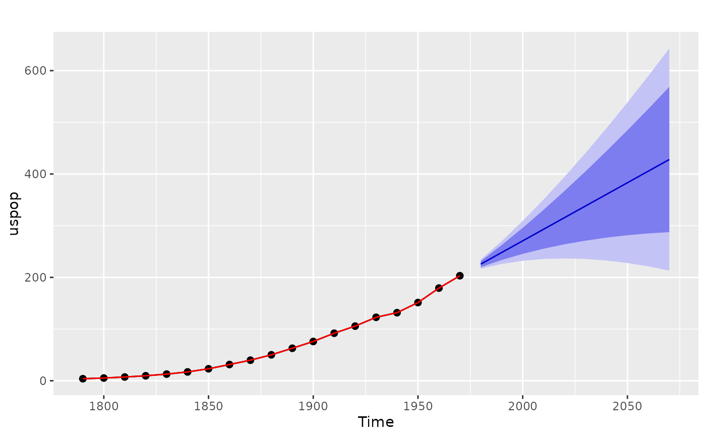
fit <- spline_model(uspop)
fcast <- forecast(fit)
autoplot(fcast)

summary(fcast)
#> 
#> Forecast method: Cubic Smoothing Spline
#> 
#> Model Information:
#> Cubic spline stochastic model
#> Call: spline_model(y = uspop) 
#> Smoothing parameter: 0.0006859 
#> 
#> Error measures:
#>                     ME     RMSE      MAE        MPE     MAPE       MASE
#> Training set 0.7704553 4.572546 3.165298 -0.6110405 8.174722 0.04536795
#>                    ACF1
#> Training set -0.4363661
#> 
#> Forecasts:
#>      Point Forecast    Lo 80    Hi 80    Lo 95    Hi 95
#> 1980       225.6937 219.8454 231.5419 216.7496 234.6378
#> 1990       248.1814 233.7246 262.6382 226.0717 270.2912
#> 2000       270.6692 245.5023 295.8361 232.1798 309.1586
#> 2010       293.1569 255.5241 330.7897 235.6025 350.7113
#> 2020       315.6447 264.0068 367.2826 236.6713 394.6181
#> 2030       338.1324 271.1025 405.1624 235.6190 440.6459
#> 2040       360.6202 276.9258 444.3146 232.6206 488.6198
#> 2050       383.1080 281.5668 484.6491 227.8141 538.4018
#> 2060       405.5957 285.0989 526.0925 221.3118 589.8797
#> 2070       428.0835 287.5834 568.5835 213.2072 642.9598

Returns local linear forecasts and prediction intervals using cubic smoothing splines estimated with `spline_model()`.