Cubic spline stochastic model

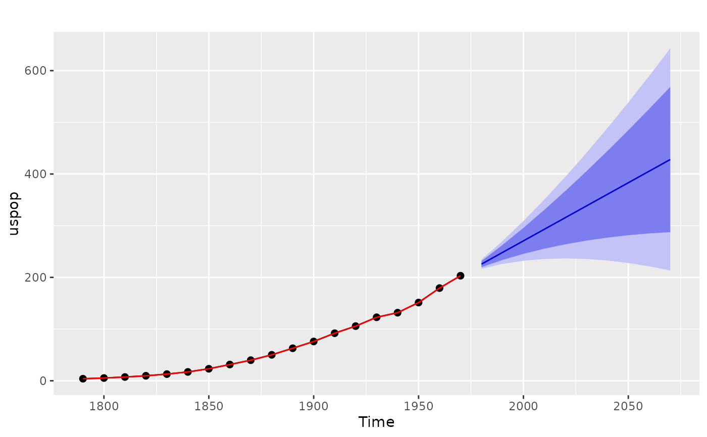
Fits a state space model based on cubic smoothing splines. The cubic smoothing spline model is equivalent to an ARIMA(0,2,2) model but with a restricted parameter space. The advantage of the spline model over the full ARIMA model is that it provides a smooth historical trend as well as a linear forecast function. Hyndman, King, Pitrun, and Billah (2002) show that the forecast performance of the method is hardly affected by the restricted parameter space.

Usage

spline_model(y, method = c("gcv", "mle"), lambda = NULL, biasadj = FALSE)

Arguments

y: a numeric vector or univariate time series of class ts
method: Method for selecting the smoothing parameter. If method = "gcv", the generalized cross-validation method from stats::smooth.spline() is used. If method = "mle", the maximum likelihood method from Hyndman et al (2002) is used.
lambda: Box-Cox transformation parameter. If lambda = "auto", then a transformation is automatically selected using BoxCox.lambda. The transformation is ignored if NULL. Otherwise, data transformed before model is estimated.
biasadj: Use adjusted back-transformed mean for Box-Cox transformations. If transformed data is used to produce forecasts and fitted values, a regular back transformation will result in median forecasts. If biasadj is TRUE, an adjustment will be made to produce mean forecasts and fitted values.

Value

An object of class spline_model.

References

Hyndman, King, Pitrun and Billah (2005) Local linear forecasts using cubic smoothing splines. Australian and New Zealand Journal of Statistics, 47(1), 87-99. https://robjhyndman.com/publications/splinefcast/.

Author

Rob J Hyndman

Examples

fit <- spline_model(uspop)
fit
#> Cubic spline stochastic model
#> Call: spline_model(y = uspop) 
#> Smoothing parameter: 0.0006859 
fit |> forecast() |> autoplot()