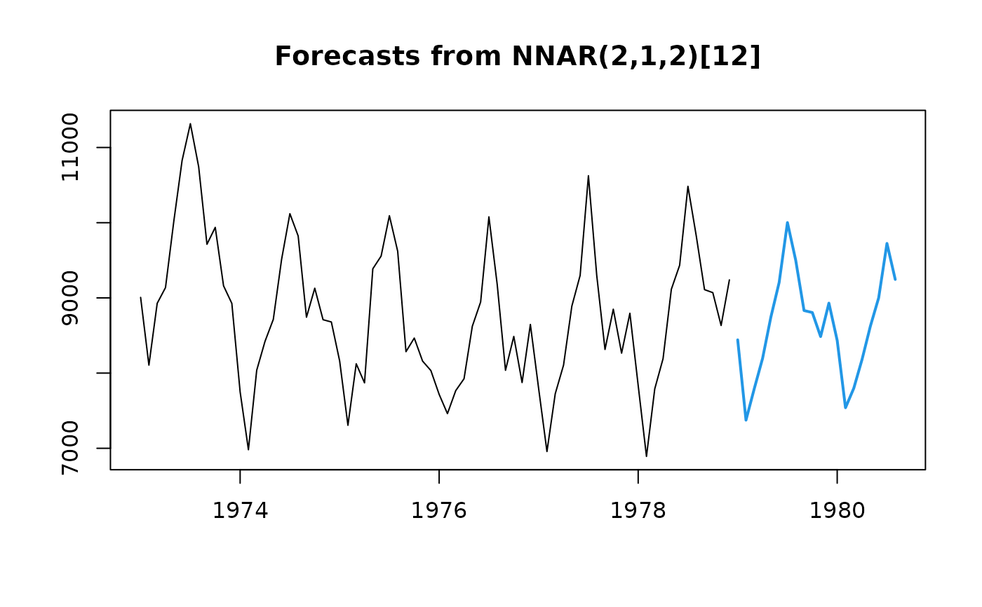
Forecasting using neural network models

Returns forecasts and other information for univariate neural network models.

Usage

# S3 method for class 'nnetar'
forecast(
  object,
  h = if (object$m > 1) 2 * object$m else 10,
  PI = FALSE,
  level = c(80, 95),
  fan = FALSE,
  xreg = NULL,
  lambda = object$lambda,
  bootstrap = FALSE,
  npaths = 1000,
  innov = NULL,
  ...
)

Arguments

object: An object of class nnetar resulting from a call to nnetar().
h: Number of periods for forecasting. If xreg is used, h is ignored and the number of forecast periods is set to the number of rows of xreg.
PI: If TRUE, prediction intervals are produced, otherwise only point forecasts are calculated. If PI is FALSE, then level, fan, bootstrap and npaths are all ignored.
level: Confidence levels for prediction intervals.
fan: If TRUE, level is set to seq(51, 99, by = 3). This is suitable for fan plots.
xreg: Future values of any regression variables. A numerical vector or matrix of external regressors; it should not be a data frame.
lambda: Box-Cox transformation parameter. If lambda = "auto", then a transformation is automatically selected using BoxCox.lambda. The transformation is ignored if NULL. Otherwise, data transformed before model is estimated.
bootstrap: If TRUE, then prediction intervals are produced by simulation using resampled errors (rather than normally distributed errors).
npaths: Number of sample paths used in computing simulated prediction intervals.
innov: Values to use as innovations for prediction intervals. Must be a matrix with h rows and npaths columns (vectors are coerced into a matrix). If present, bootstrap is ignored.
...: Additional arguments passed to simulate.nnetar().

Value

An object of class forecast.

Details

Prediction intervals are calculated through simulations and can be slow. Note that if the network is too complex and overfits the data, the residuals can be arbitrarily small; if used for prediction interval calculations, they could lead to misleadingly small values. It is possible to use out-of-sample residuals to ameliorate this, see examples.

forecast class

An object of class forecast is a list usually containing at least the following elements:

model: A list containing information about the fitted model
method: The name of the forecasting method as a character string
mean: Point forecasts as a time series
lower: Lower limits for prediction intervals
upper: Upper limits for prediction intervals
level: The confidence values associated with the prediction intervals
x: The original time series.
residuals: Residuals from the fitted model. For models with additive errors, the residuals will be x minus the fitted values.
fitted: Fitted values (one-step forecasts)

The function summary can be used to obtain and print a summary of the results, while the functions plot and autoplot produce plots of the forecasts and prediction intervals. The generic accessors functions fitted.values and residuals extract various useful features from the underlying model.

Author

Rob J Hyndman and Gabriel Caceres

Examples

## Fit & forecast model
fit <- nnetar(USAccDeaths, size = 2)
fcast <- forecast(fit, h = 20)
plot(fcast)


if (FALSE) { # \dontrun{
## Include prediction intervals in forecast
fcast2 <- forecast(fit, h = 20, PI = TRUE, npaths = 100)
plot(fcast2)

## Set up out-of-sample innovations using cross-validation
fit_cv <- CVar(USAccDeaths, size = 2)
res_sd <- sd(fit_cv$residuals, na.rm = TRUE)
myinnovs <- rnorm(20 * 100, mean = 0, sd = res_sd)
## Forecast using new innovations
fcast3 <- forecast(fit, h = 20, PI = TRUE, npaths = 100, innov = myinnovs)
plot(fcast3)
} # }