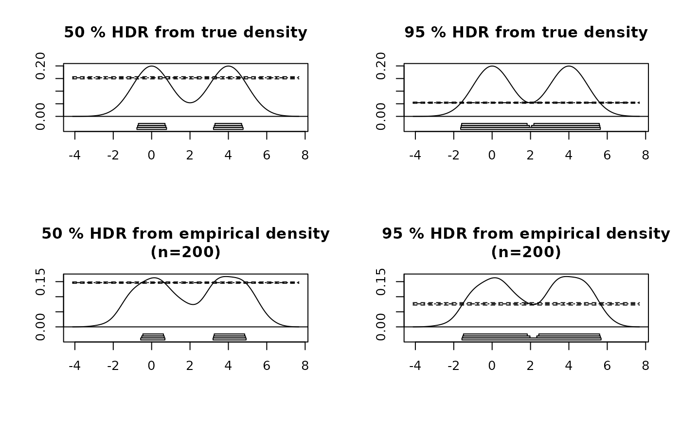
Plots Highest Density Regions with confidence intervals.
Usage
# S3 method for class 'hdrconf'
plot(x, den, ...)References
Hyndman, R.J. (1996) Computing and graphing highest density regions American Statistician, 50, 120-126.
Examples
x <- c(rnorm(100, 0, 1), rnorm(100, 4, 1))
den <- density(x, bw = bw.SJ(x))
trueden <- den
trueden$y <- 0.5 * (exp(-0.5 * (den$x * den$x)) + exp(-0.5 * (den$x - 4)^2)) / sqrt(2 * pi)

par(mfcol = c(2, 2))
for (conf in c(50, 95)) {
  m <- hdrconf(x, trueden, conf = conf)
  plot(m, trueden, main = paste(conf, "% HDR from true density"))
  m <- hdrconf(x, den, conf = conf)
  plot(m, den, main = paste(conf, "% HDR from empirical density\n(n=200)"))
}