Time series display

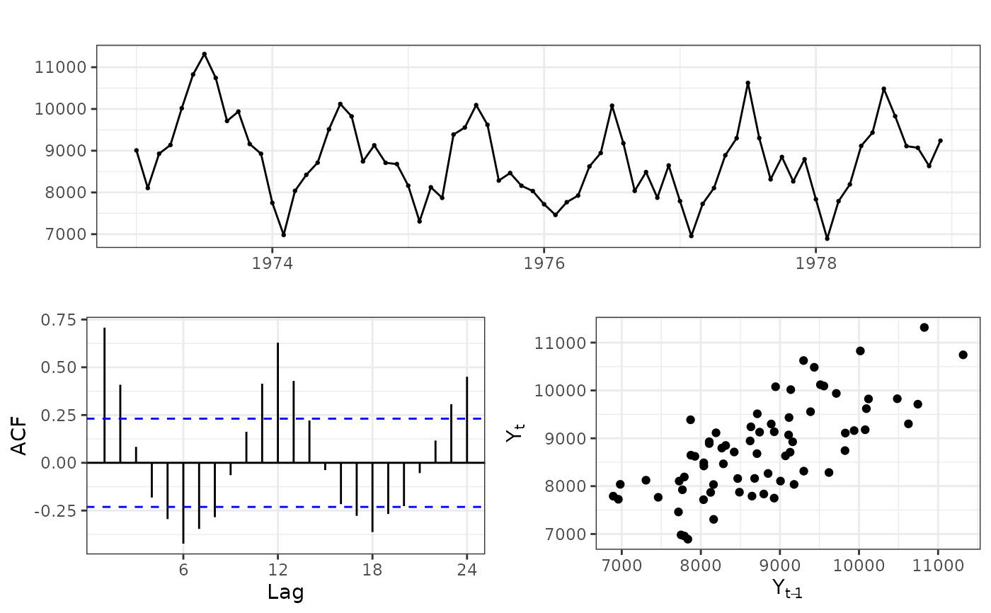
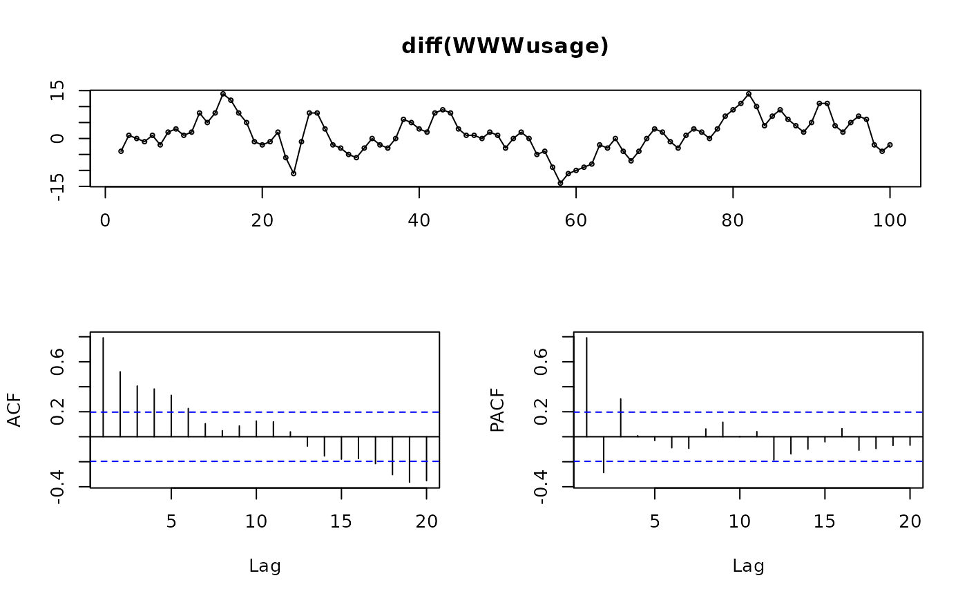
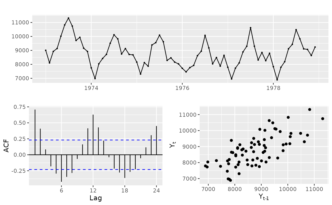
Plots a time series along with its acf and either its pacf, lagged scatterplot or spectrum.

Usage

ggtsdisplay(
  x,
  plot.type = c("partial", "histogram", "scatter", "spectrum"),
  points = TRUE,
  smooth = FALSE,
  lag.max,
  na.action = na.contiguous,
  theme = NULL,
  ...
)

tsdisplay(
  x,
  plot.type = c("partial", "histogram", "scatter", "spectrum"),
  points = TRUE,
  ci.type = c("white", "ma"),
  lag.max,
  na.action = na.contiguous,
  main = NULL,
  xlab = "",
  ylab = "",
  pch = 1,
  cex = 0.5,
  ...
)

Arguments

x: a numeric vector or time series of class ts.
plot.type: type of plot to include in lower right corner.
points: logical flag indicating whether to show the individual points or not in the time plot.
smooth: logical flag indicating whether to show a smooth loess curve superimposed on the time plot.
lag.max: the maximum lag to plot for the acf and pacf. A suitable value is selected by default if the argument is missing.
na.action: function to handle missing values in acf, pacf and spectrum calculations. The default is na.contiguous. Useful alternatives are na.pass and na.interp.
theme: Adds a ggplot element to each plot, typically a theme.
...: additional arguments to acf.
ci.type: type of confidence limits for ACF that is passed to acf. Should the confidence limits assume a white noise input or for lag \(k\) an MA(\(k-1\)) input?
main: Main title.
xlab: X-axis label.
ylab: Y-axis label.
pch: Plotting character.
cex: Character size.

Value

None.

Details

ggtsdisplay will produce the equivalent plot using ggplot graphics.

References

Hyndman and Athanasopoulos (2018) Forecasting: principles and practice, 2nd edition, OTexts: Melbourne, Australia. https://otexts.com/fpp2/

Author

Rob J Hyndman

Examples

library(ggplot2)
ggtsdisplay(USAccDeaths, plot.type="scatter", theme=theme_bw())


tsdisplay(diff(WWWusage))

ggtsdisplay(USAccDeaths, plot.type="scatter")