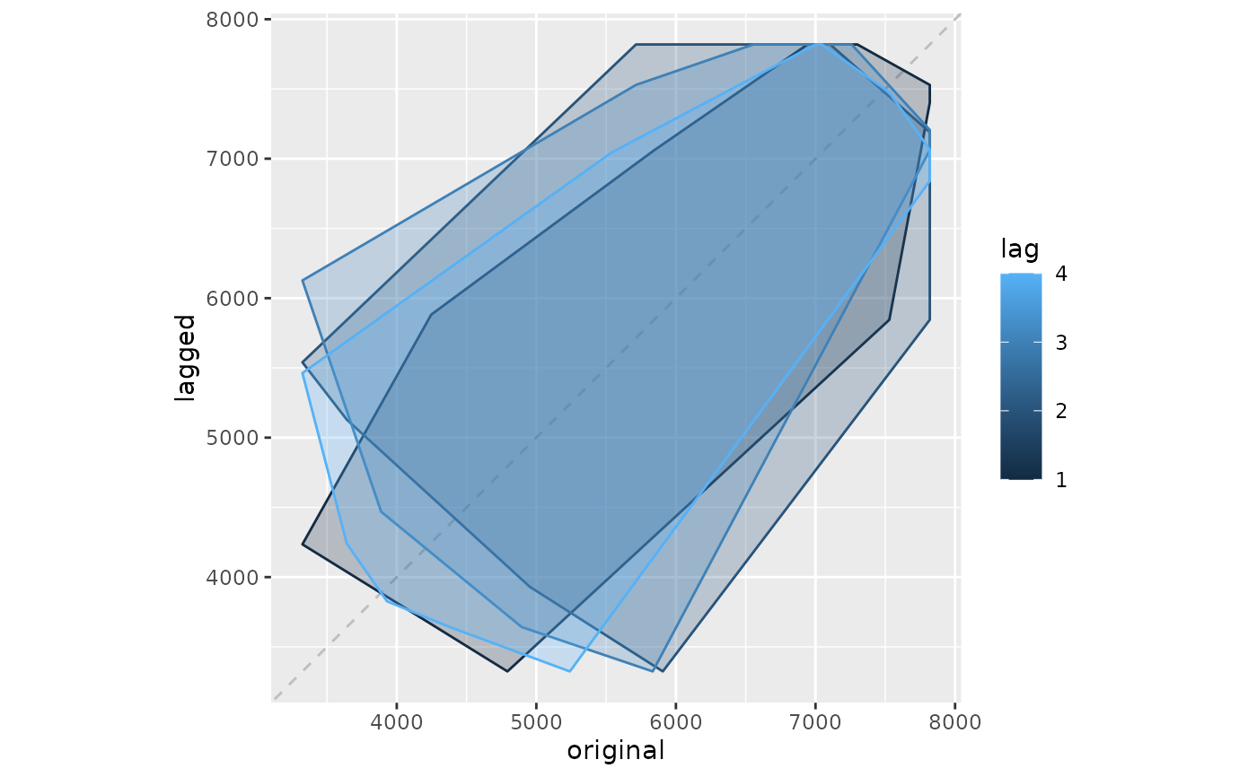
Plots a lag plot using ggplot.
Usage
gglagplot(
  x,
  lags = if (frequency(x) > 9) 16 else 9,
  set.lags = 1:lags,
  diag = TRUE,
  diag.col = "gray",
  do.lines = TRUE,
  colour = TRUE,
  continuous = frequency(x) > 12,
  labels = FALSE,
  seasonal = TRUE,
  ...
)

gglagchull(
  x,
  lags = if (frequency(x) > 1) min(12, frequency(x)) else 4,
  set.lags = 1:lags,
  diag = TRUE,
  diag.col = "gray",
  ...
)
Arguments
- x
a time series object (type
ts).- lags
number of lag plots desired, see arg set.lags.
- set.lags
vector of positive integers specifying which lags to use.
- diag
logical indicating if the x=y diagonal should be drawn.
- diag.col
color to be used for the diagonal if(diag).
- do.lines
if
TRUE, lines will be drawn, otherwise points will be drawn.- colour
logical indicating if lines should be coloured.
- continuous
Should the colour scheme for years be continuous or discrete?
- labels
logical indicating if labels should be used.
- seasonal
Should the line colour be based on seasonal characteristics (
TRUE), or sequential (FALSE).- ...
Not used (for consistency with lag.plot)
Details
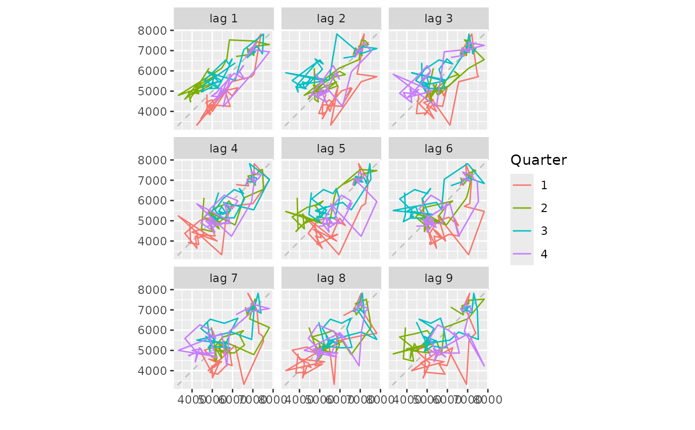
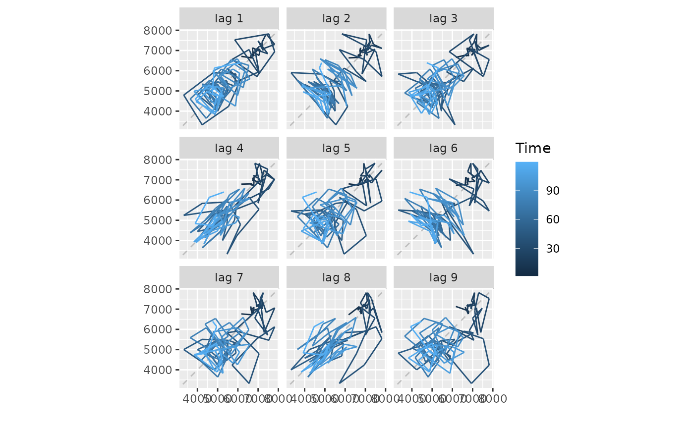
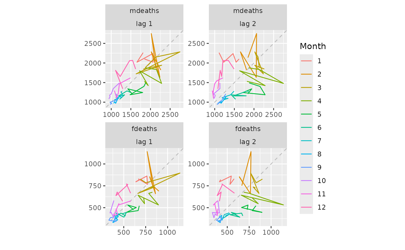
"gglagplot" will plot time series against lagged versions of themselves. Helps visualising 'auto-dependence' even when auto-correlations vanish.
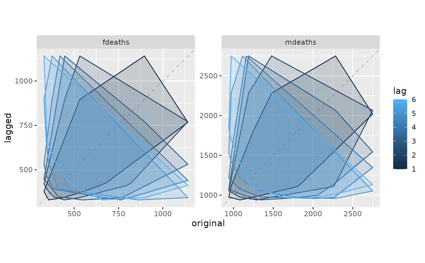
"gglagchull" will layer convex hulls of the lags, layered on a single plot. This helps visualise the change in 'auto-dependence' as lags increase.
Examples
gglagplot(woolyrnq)
 gglagplot(woolyrnq, seasonal = FALSE)
 lungDeaths <- cbind(mdeaths, fdeaths)
gglagplot(lungDeaths, lags = 2)
 gglagchull(lungDeaths, lags = 6)
 gglagchull(woolyrnq)
