Croston forecast model

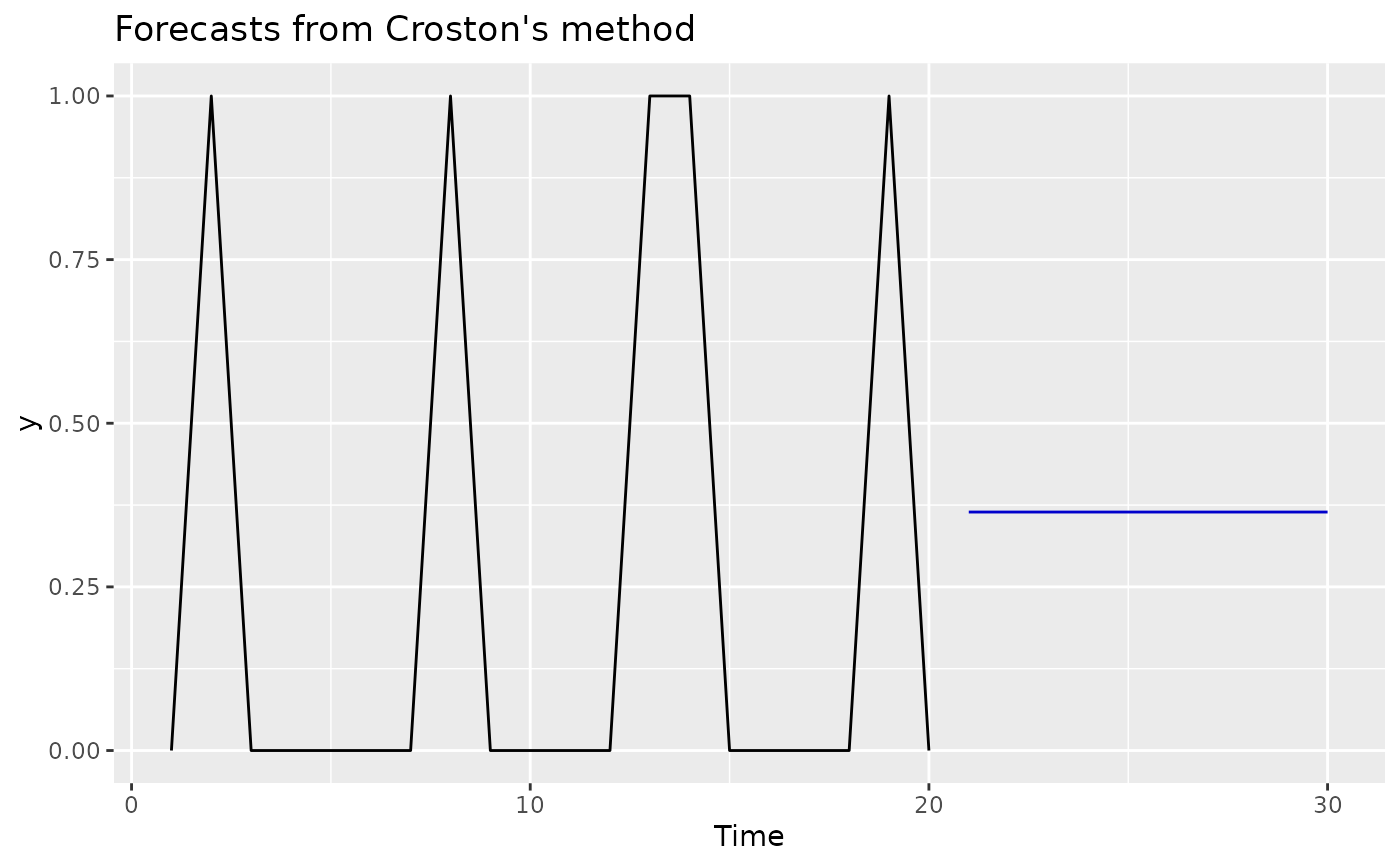
Based on Croston's (1972) method for intermittent demand forecasting, also described in Shenstone and Hyndman (2005). Croston's method involves using simple exponential smoothing (SES) on the non-zero elements of the time series and a separate application of SES to the times between non-zero elements of the time series. Returns a model object that can be used to generate forecasts using Croston's method for intermittent demand time series. It isn't a true statistical model in that it doesn't describe a data generating process that would lead to the forecasts produced using Croston's method.

Usage

croston_model(
  y,
  alpha = 0.1,
  type = c("croston", "sba", "sbj"),
  opt_alpha = FALSE,
  opt_crit = c("mse", "mae"),
  init = c("naive", "mean")
)

Arguments

y

a numeric vector or univariate time series of class ts

alpha

Smoothing parameter(s), each between 0 and 1. A single value (the default, 0.1) is shared by the demand and interval SES applications. A length-2 vector uses alpha[1] for the demand and alpha[2] for the interval.

type

Which variant of Croston's method to use. Defaults to "croston" for Croston's method, but can also be set to "sba" for the Syntetos-Boylan approximation, and "sbj" for the Shale-Boylan-Johnston method.

opt_alpha

If TRUE, optimize the smoothing parameter(s) starting from alpha. Defaults to FALSE, which uses alpha directly.

opt_crit

Optimization criterion when opt_alpha = TRUE. One of "mse" (mean squared error) or "mae" (mean absolute error).

init

Initial demand and interval values. Either a string method or a length-2 numeric c(demand, interval). The "naive" method (the default) takes the interval from the first interval and "mean" from the mean interval, both taking demand from the first non-zero value. String values are optimized alongside alpha when opt_alpha = TRUE, while numeric values are held fixed.

Value

An object of class croston_model

Details

Note that prediction intervals are not computed as Croston's method has no underlying stochastic model.

There are two variant methods available which apply multiplicative correction factors to the forecasts that result from the original Croston's method. For the Syntetos-Boylan approximation (type = "sba"), this factor is \(1 - \alpha / 2\), and for the Shale-Boylan-Johnston method (type = "sbj"), this factor is \(1 - \alpha / (2 - \alpha)\), where \(\alpha\) is the smoothing parameter for the interval SES application.

References

Croston, J. (1972) "Forecasting and stock control for intermittent demands", Operational Research Quarterly, 23(3), 289-303.

Shale, E.A., Boylan, J.E., & Johnston, F.R. (2006). Forecasting for intermittent demand: the estimation of an unbiased average. Journal of the Operational Research Society, 57(5), 588-592.

Shenstone, L., and Hyndman, R.J. (2005) "Stochastic models underlying Croston's method for intermittent demand forecasting". Journal of Forecasting, 24, 389-402.

Syntetos A.A., Boylan J.E. (2001). On the bias of intermittent demand estimates. International Journal of Production Economics, 71, 457–466.

Author

Rob J Hyndman

Examples

y <- rpois(20, lambda = 0.3)
fit <- croston_model(y)
forecast(fit) |> autoplot()