Plots the varying beta coefficients of decomposition

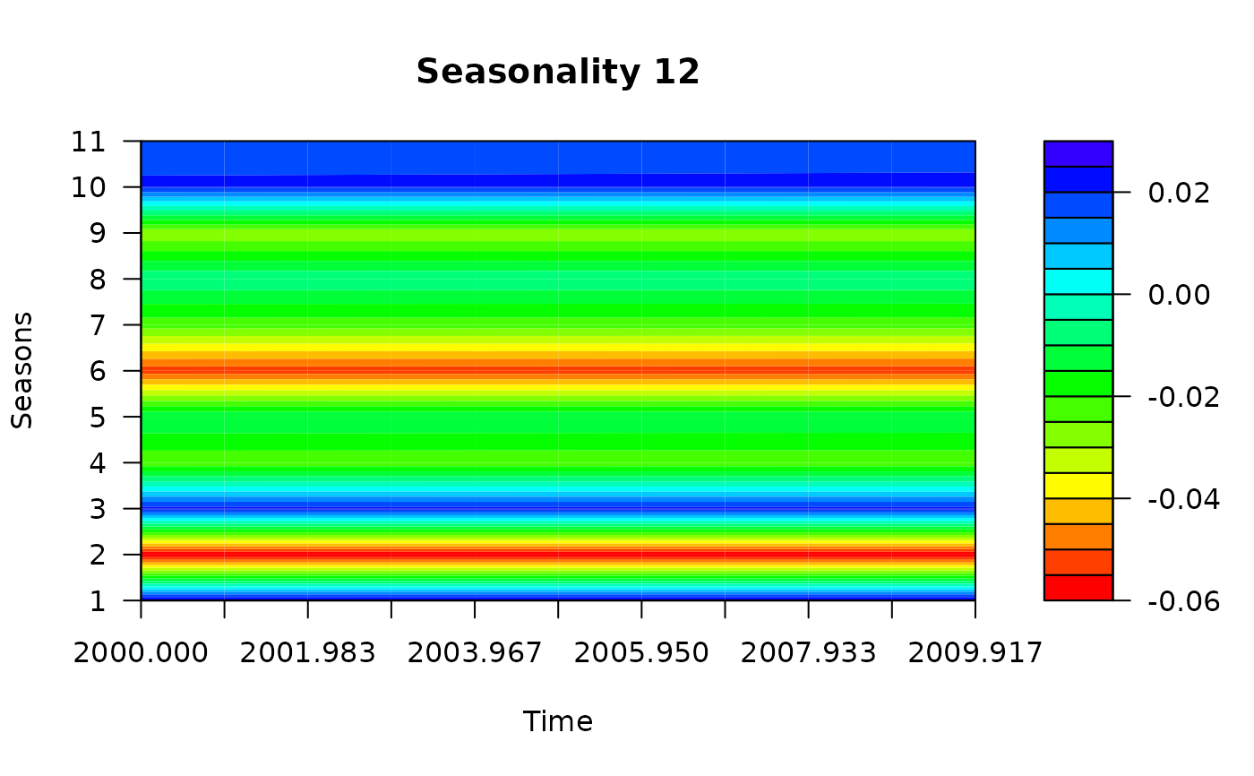
plotBeta plots the varying beta coefficients of STR decomposition. It plots coefficients only only for independent seasons (one less season than defined).

Usage

plotBeta(
  x,
  xTime = NULL,
  predictorN = 1,
  dim = c(1, 2, 3),
  type = "o",
  pch = 20,
  palette = function(n) rainbow(n, start = 0, end = 0.7)
)

Arguments

x

Result of STR decomposition.

xTime

Times for data to plot.

predictorN

Predictor number in the decomposition to plot the corresponding beta coefficiets.

dim

Dimensions to use to plot the beta coefficients. When 1, the standard charts are used. When 2, graphics:::filled.contour function is used. When 3, rgl:::persp3d is used. The default value is 1.

type

Type of the graph for one dimensional plots.

pch

Symbol code to plot points in 1-dimensional charts. Default value is 20.

palette

Color palette for 2 - and 3 - dimentional plots.

See also

plot.STR

Author

Alexander Dokumentov

Examples

# \donttest{
fit <- AutoSTR(log(grocery))
for (i in 1:2) plotBeta(fit, predictorN = i, dim = 2)



########################################

TrendSeasonalStructure <- list(
  segments = list(c(0, 1)),
  sKnots = list(c(1, 0))
)
DailySeasonalStructure <- list(
  segments = list(c(0, 48)),
  sKnots = c(as.list(1:47), list(c(48, 0)))
)
WeeklySeasonalStructure <- list(
  segments = list(c(0, 336)),
  sKnots = c(as.list(seq(4, 332, 4)), list(c(336, 0)))
)
WDSeasonalStructure <- list(
  segments = list(c(0, 48), c(100, 148)),
  sKnots = c(as.list(c(1:47, 101:147)), list(c(0, 48, 100, 148)))
)

TrendSeasons <- rep(1, nrow(electricity))
DailySeasons <- as.vector(electricity[, "DailySeasonality"])
WeeklySeasons <- as.vector(electricity[, "WeeklySeasonality"])
WDSeasons <- as.vector(electricity[, "WorkingDaySeasonality"])

Data <- as.vector(electricity[, "Consumption"])
Times <- as.vector(electricity[, "Time"])
TempM <- as.vector(electricity[, "Temperature"])
TempM2 <- TempM^2

TrendTimeKnots <- seq(from = head(Times, 1), to = tail(Times, 1), length.out = 116)
SeasonTimeKnots <- seq(from = head(Times, 1), to = tail(Times, 1), length.out = 24)
SeasonTimeKnots2 <- seq(from = head(Times, 1), to = tail(Times, 1), length.out = 12)

TrendData <- rep(1, length(Times))
SeasonData <- rep(1, length(Times))

Trend <- list(
  name = "Trend",
  data = TrendData,
  times = Times,
  seasons = TrendSeasons,
  timeKnots = TrendTimeKnots,
  seasonalStructure = TrendSeasonalStructure,
  lambdas = c(1500, 0, 0)
)
WSeason <- list(
  name = "Weekly seas",
  data = SeasonData,
  times = Times,
  seasons = WeeklySeasons,
  timeKnots = SeasonTimeKnots2,
  seasonalStructure = WeeklySeasonalStructure,
  lambdas = c(0.8, 0.6, 100)
)
WDSeason <- list(
  name = "Dayly seas",
  data = SeasonData,
  times = Times,
  seasons = WDSeasons,
  timeKnots = SeasonTimeKnots,
  seasonalStructure = WDSeasonalStructure,
  lambdas = c(0.003, 0, 240)
)
TrendTempM <- list(
  name = "Trend temp Mel",
  data = TempM,
  times = Times,
  seasons = TrendSeasons,
  timeKnots = TrendTimeKnots,
  seasonalStructure = TrendSeasonalStructure,
  lambdas = c(1e7, 0, 0)
)
TrendTempM2 <- list(
  name = "Trend temp Mel^2",
  data = TempM2,
  times = Times,
  seasons = TrendSeasons,
  timeKnots = TrendTimeKnots,
  seasonalStructure = TrendSeasonalStructure,
  lambdas = c(0.01, 0, 0)
) # Starting parameter is too far from the optimal value
Predictors <- list(Trend, WSeason, WDSeason, TrendTempM, TrendTempM2)

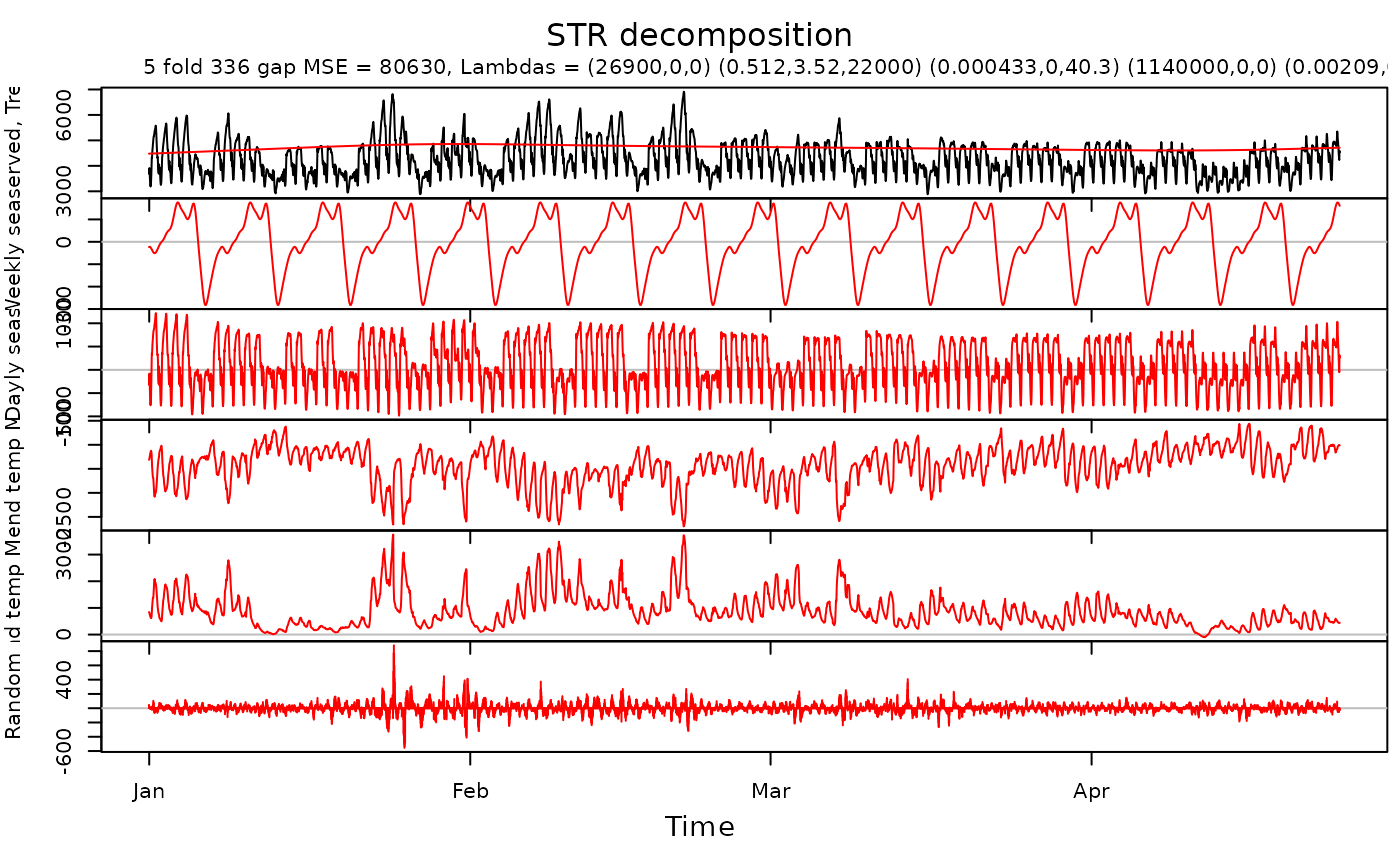
elec.fit <- STR(
  data = Data,
  predictors = Predictors,
  gapCV = 48 * 7
)

plot(elec.fit,
  xTime = as.Date("2000-01-11") + ((Times - 1) / 48 - 10),
  forecastPanels = NULL
)


plotBeta(elec.fit, predictorN = 4)

plotBeta(elec.fit, predictorN = 5) # Beta coefficients are too "wiggly"

# }