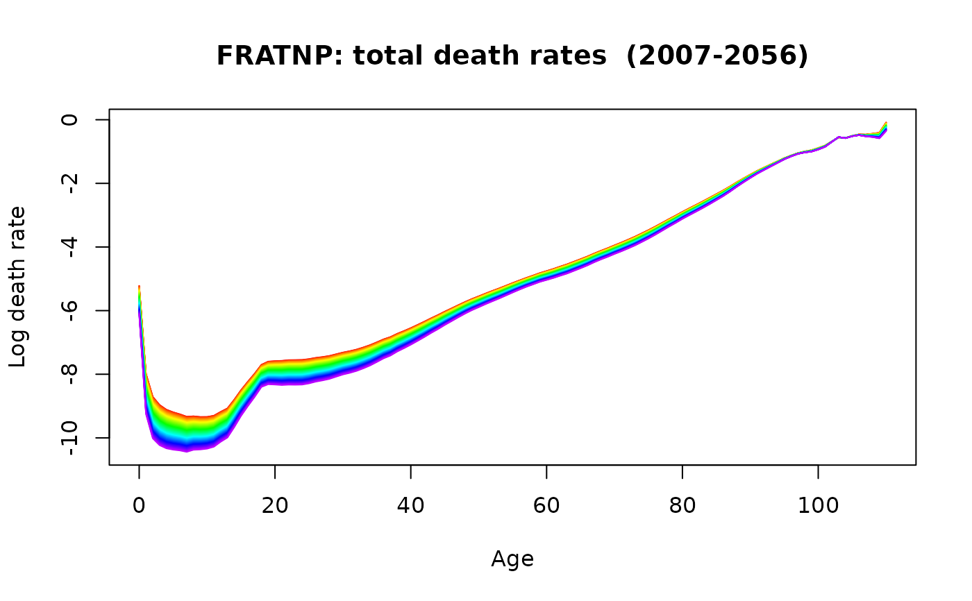
The coefficients from the fitted object are forecast using a univariate time series model. The forecast coefficients are then multiplied by the basis functions to obtain a forecast demographic rate curve.
Usage
# S3 method for class 'fdm'
forecast(
  object,
  h = 50,
  level = 80,
  jumpchoice = c("fit", "actual"),
  method = "arima",
  warnings = FALSE,
  ...
)
Arguments
- object
Output from
fdm.- h
Forecast horizon.
- level
Confidence level for prediction intervals.
- jumpchoice
If "actual", the forecasts are bias-adjusted by the difference between the fit and the last year of observed data. Otherwise, no adjustment is used.
- method
Forecasting method to be used.
- warnings
If TRUE, warnings arising from the forecast models for coefficients will be shown. Most of these can be ignored, so the default is
warnings=FALSE.- ...
Other arguments as for
forecast.ftsm.
Value
Object of class fmforecast with the following components:
- label
Name of region from which the data are taken.
- age
Ages from
lcaoutobject.- year
Years from
lcaoutobject.- rate
List of matrices containing forecasts, lower bound and upper bound of prediction intervals. Point forecast matrix takes the same name as the series that has been forecast.
- error
Matrix of one-step errors for historical data
- fitted
Matrix of one-step forecasts for historical data
- coeff
List of objects of type
forecastcontaining the coefficients and their forecasts.- coeff.error
One-step errors for each of the coefficients.
- var
List containing the various components of variance: model, error, mean, total and coeff.
- model
Fitted model in
obj.- type
Type of data: “mortality”, “fertility” or “migration”.
Examples
france.fit <- fdm(fr.mort, order = 2)
france.fcast <- forecast(france.fit, 50)
plot(france.fcast)

models(france.fcast)
#>
#> -- Coefficient 1 --
#> Series: xx[, i]
#> ARIMA(1,1,1) with drift
#>
#> Coefficients:
#>          ar1      ma1    drift
#>       0.6383  -0.8145  -0.1265
#> s.e.  0.1481   0.1120   0.0411
#>
#> sigma^2 = 1.206:  log likelihood = -285.97
#> AIC=579.95   AICc=580.16   BIC=592.93
#>
#> -- Coefficient 2 --
#> Series: xx[, i]
#> ARIMA(2,1,1)
#>
#> Coefficients:
#>          ar1     ar2      ma1
#>       0.3818  0.2926  -0.9679
#> s.e.  0.0758  0.0745   0.0280
#>
#> sigma^2 = 0.9067:  log likelihood = -259.4
#> AIC=526.79   AICc=527.01   BIC=539.78