Produce ggplot of densities from kde objects in 1 or 2 dimensions

Usage

# S3 method for class 'kde'
autoplot(
  object,
  prob = seq(9)/10,
  fill = FALSE,
  show_hdr = FALSE,
  show_points = FALSE,
  show_mode = FALSE,
  show_lookout = FALSE,
  color = "#00659e",
  alpha = ifelse(fill, 1, min(1, 1000/NROW(object$x))),
  ...
)

Arguments

object: Probability density function as estimated by ks::kde().
prob: Probability of the HDR contours to be drawn (for a bivariate plot only).
fill: If TRUE, and the density is bivariate, the bivariate contours are shown as filled regions rather than lines.
show_hdr: If TRUE, and the density is univariate, then the HDR regions specified by prob are shown as a ribbon below the density.
show_points: If TRUE, then individual points are plotted.
show_mode: If TRUE, then the mode of the distribution is shown.
show_lookout: If TRUE, then the observations with lookout probabilities less than 0.05 are shown in red.
color: Color used for mode and HDR contours. If fill, this is the base color used in constructing the palette.
alpha: Transparency of points. When fill is FALSE, defaults to min(1, 1000/n), where n is the number of observations. Otherwise, set to 1.
...: Additional arguments are currently ignored.

Value

A ggplot object.

Details

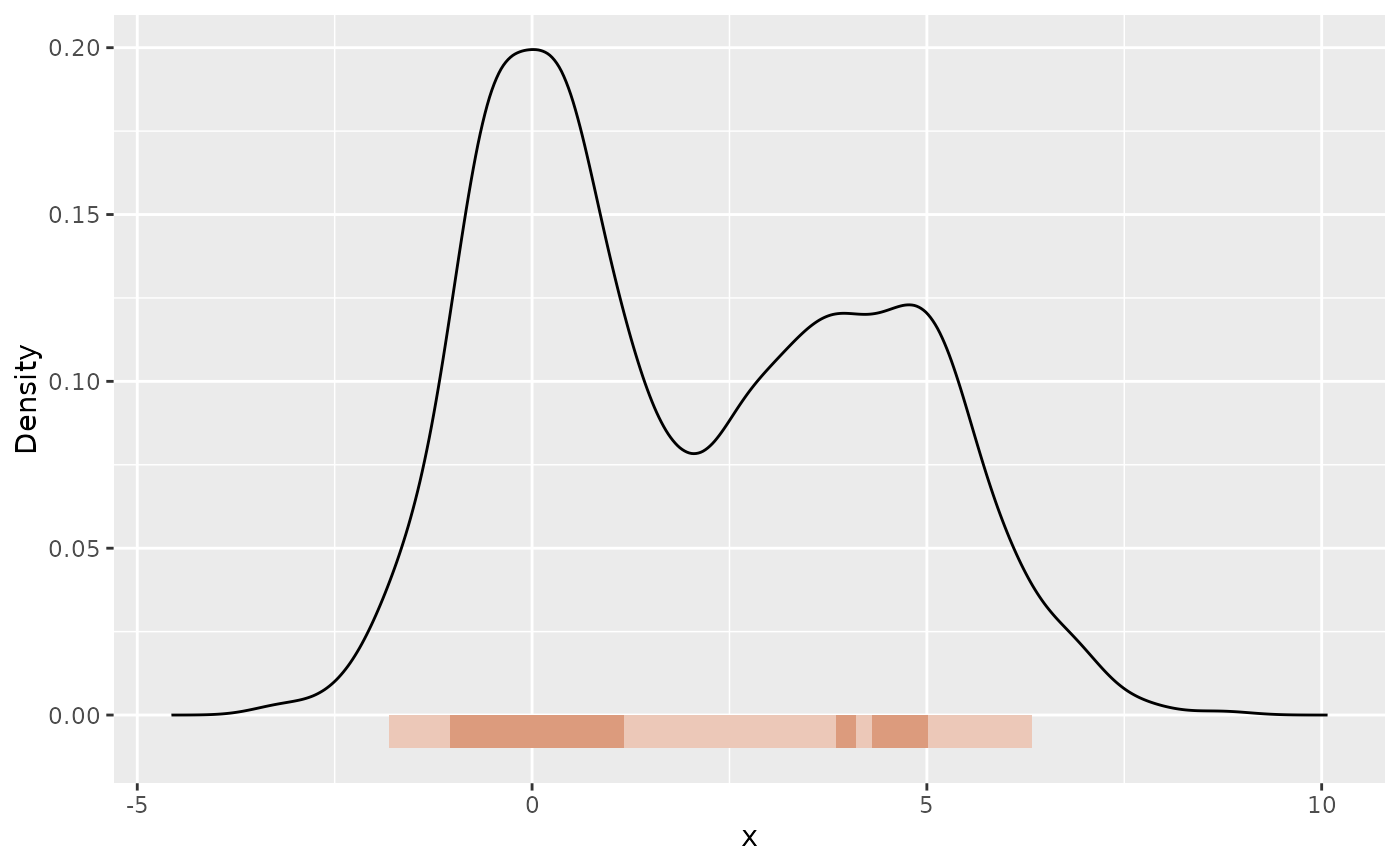
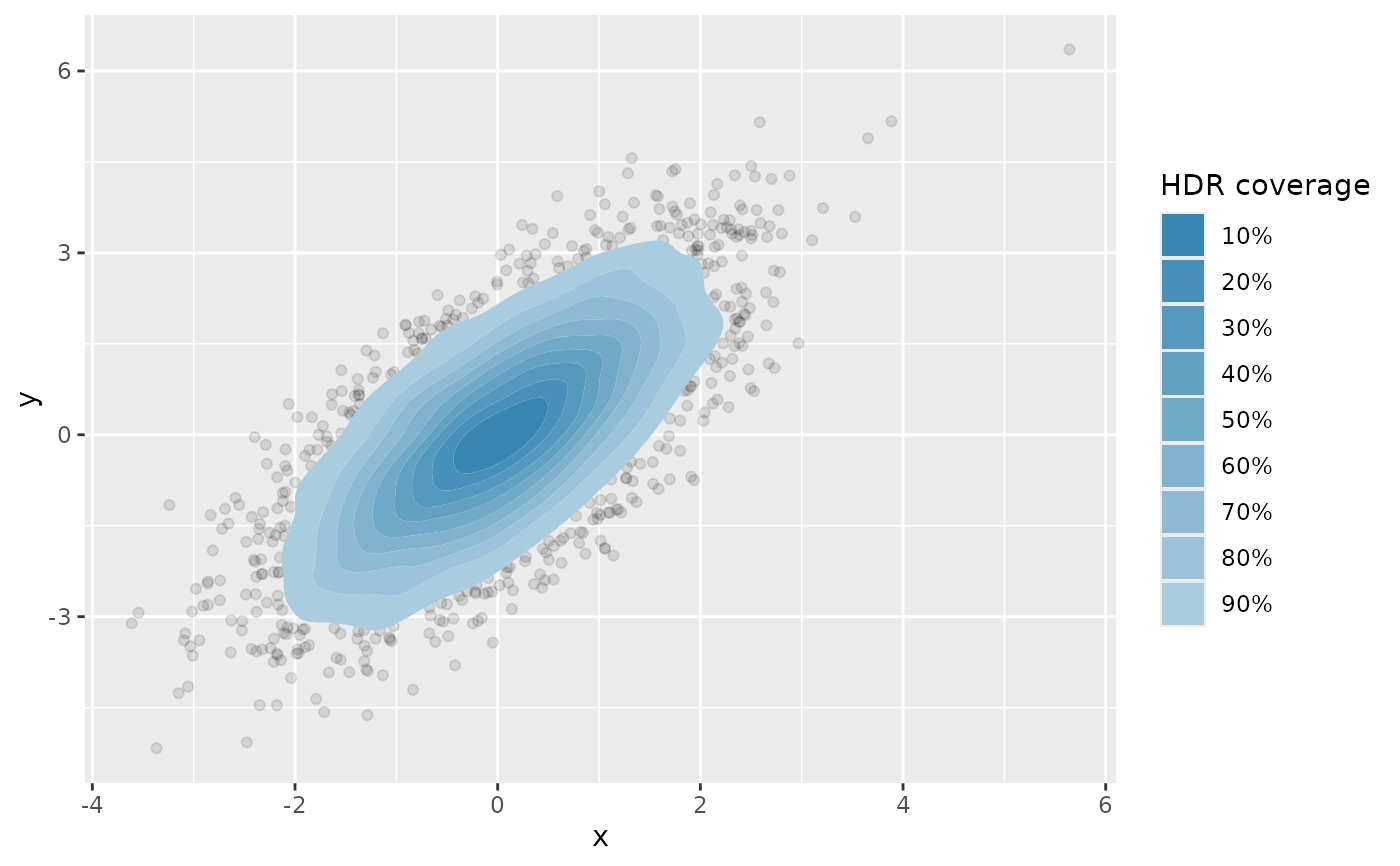
This function produces a ggplot of the density estimate produced by ks::kde(). For univariate densities, it produces a line plot of the density function, with an optional ribbon showing some highest density regions (HDRs) and/or the observations. For bivariate densities, it produces a contour plot of the density function, with the observations optionally shown as points. The mode can also be drawn as a point with the HDRs. For bivariate densities, the combination of fill = TRUE, show_points = TRUE, show_mode = TRUE, and prob = c(0.5, 0.99) is equivalent to an HDR boxplot. For univariate densities, the combination of show_hdr = TRUE, show_points = TRUE, show_mode = TRUE, and prob = c(0.5, 0.99) is equivalent to an HDR boxplot.

Author

Rob J Hyndman

Examples

# Univariate density
c(rnorm(500), rnorm(500, 4, 1.5)) |>
  ks::kde() |>
  autoplot(show_hdr = TRUE, prob = c(0.5, 0.95), color = "#c14b14")

ymat <- tibble(y1 = rnorm(5000), y2 = y1 + rnorm(5000))
ymat |>
  ks::kde(H = kde_bandwidth(ymat)) |>
  autoplot(show_points = TRUE, alpha = 0.1, fill = TRUE)