Nonparametric Multimodal Regression

Nonparametric multi-valued regression based on the modes of conditional density estimates.

Usage

modalreg(
  x,
  y,
  xfix = seq(min(x), max(x), l = 50),
  a,
  b,
  deg = 0,
  iter = 30,
  P = 2,
  start = "e",
  prun = TRUE,
  prun.const = 10,
  plot.type = c("p", 1),
  labels = c("", "x", "y"),
  pch = 20,
  ...
)

Arguments

x: Numerical vector: the conditioning variable.
y: Numerical vector: the response variable.
xfix: Numerical vector corresponding to the input values of which the fitted values shall be calculated.
a: Optional bandwidth in \(x\)-direction.
b: Optional bandwidth in \(y\)-direction.
deg: Degree of local polynomial used in estimation (0 or 1).
iter: Positive integer giving the number of mean shift iterations per point and branch.
P: Maximal number of branches.
start: Character determining how the starting points are selected. "q": proportional to quantiles; "e": equidistant; "r": random. All, "q", "e", and "r", give starting points which are constant over x. As an alternative, the choice "v" gives variable starting points, which are equal to "q" for the smallest x, and equal to the previously fitted values for all subsequent x.
prun: Boolean. If TRUE, parts of branches are dismissed (in the plotted output) where their associated kernel density value falls below the threshold 1/(prun.const*(max(x)-min(x))*(max(y)-min(y))).
prun.const: Numerical value giving the constant used above (the higher, the less pruning)
plot.type: Vector with two elements. The first one is character-valued, with possible values "p", "l", and "n". If equal to "n", no plotted output is given at all. If equal to "p", fitted curves are symbolized as points in the graphical output, otherwise as lines. The second vector component is a numerical value either being 0 or 1. If 1, the position of the starting points is depicted in the plot, otherwise omitted.
labels: Vector of three character strings. The first one is the "main" title of the graphical output, the second one is the label of the \(x\) axis, and the third one the label of the \(y\) axis.
pch: Plotting character. The default corresponds to small bullets.
...: Other arguments passed to cde.bandwidths.

Value

A list with the following components:

xfix: Grid of predictor values at which the fitted values are calculated.
fitted.values: A [P x length(xfix)]- matrix with fitted j-th branch in the j-th row (\(1 \le j \le P\))
bandwidths: A vector with bandwidths a and b.
density: A [P x length(xfix)]- matrix with estimated kernel densities. This will only be computed if prun=TRUE.
threshold: The pruning threshold.

Details

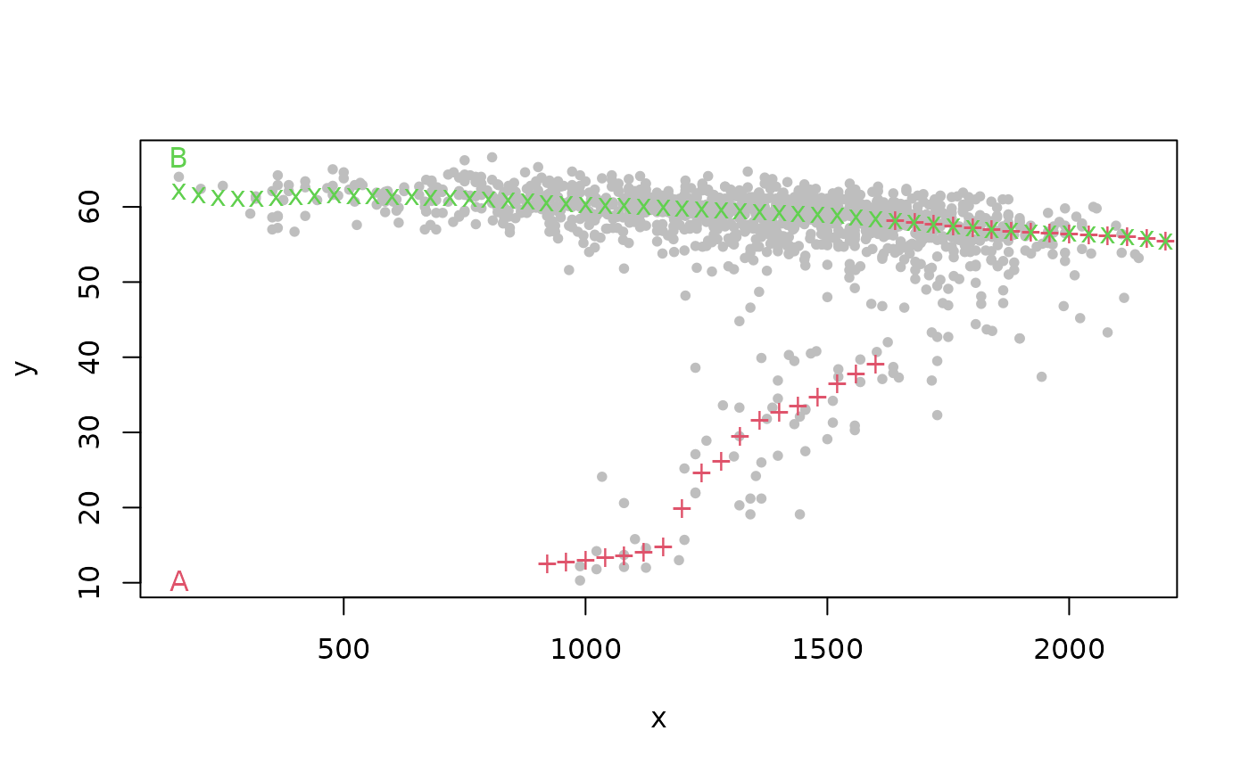
Computes multi-modal nonparametric regression curves based on the maxima of conditional density estimates. The tool for the estimation is the conditional mean shift as outlined in Einbeck and Tutz (2006). Estimates of the conditional modes might fluctuate highly if deg=1. Hence, deg=0 is recommended. For bandwidth selection, the hybrid rule introduced by Bashtannyk and Hyndman (2001) is employed if deg=0. This corresponds to the setting method=1 in function cde.bandwidths. For deg=1 automatic bandwidth selection is not supported.

References

Einbeck, J., and Tutz, G. (2006) "Modelling beyond regression functions: an application of multimodal regression to speed-flow data". Journal of the Royal Statistical Society, Series C (Applied Statistics), 55, 461-475.

Bashtannyk, D.M., and Hyndman, R.J. (2001) "Bandwidth selection for kernel conditional density estimation". Computational Statistics and Data Analysis, 36(3), 279-298.

Author

Jochen Einbeck (2007)

Examples

lane2.fit <- modalreg(lane2$flow, lane2$speed, xfix=(1:55)*40, a=100, b=4)

#> 10 ..20 ..30 ..40 ..50 ..